SSSP is one of the most frequent graph problem encountered in real-life. Every time we want to move from one place (usually our current location) to another (our destination), we will try to pick a short — if not the shortest — path.

SSSP algorithm(s) is embedded inside various map software like Google Maps and in various Global Positioning System (GPS) tool.

Input 1: A directed weighted graph G(V, E), not necessarily connected, where V/vertices can be used to describe intersections, junctions, houses, landmarks, etc and E/edges can be used to describe streets, roads, avenues with proper direction and weight/cost.

Input 2: As the name implies, the SSSP problem has another input: A source vertex s ∈ V.

The objective of the SSSP problem is to find the shortest path weight from s to each vertex u ∈ V, denoted as δ(s, u) (δ is pronounced as 'delta') and also the actual shortest path from s to u.

The path weight of a path p is simply the summation of edge weights along that path.

The weight of the shortest path from s to s is trivial: 0.
The weight of the shortest path from s to any unreachable vertex is also trivial: +∞.

PS: The weight of the shortest path from s to v where (s, v) ∈ E does not necessarily the weight of w(s, v). See the next few slides to realise this.

在这个可视化中讨论的所有六种（6）SSSP算法的输出结果是这两个数组/向量：

1. 一个大小为V的数组/向量D（D代表 'distance'）
   最初，如果u = s，那么D[u] = 0；否则D[u] = +∞（一个大数，例如 10⁹）
   当我们找到更好（更短）的路径时，D[u]会减小
   在SSSP算法的执行过程中，D[u] ≥ δ(s, u)
   在SSSP算法结束时，D[u] = δ(s, u)
2. 一个大小为V的数组/向量p（p代表 'parent'/'predecessor'/'previous'）
   p[u] = 来源s到u的最佳路径上的前驱
   p[u] = NULL（未定义，我们可以使用像-1这样的值）
   这个数组/向量p描述了结果SSSP生成树

最初，D[u] = +∞ (实际上，一个大的值，如 10⁹) ∀u ∈ V\\{s}，但 D[s] = D[0] = 0。
最初，p[u] = -1 (表示 '没有前驱') ∀u ∈ V。

现在点击 Dijkstra(0) —— 不用担心细节，稍后会解释 —— 等待结束 (在这个小图上大约需要10秒)。

在那个SSSP算法结束时，D[s] = D[0] = 0 (未改变) 和 D[u] = δ(s, u) ∀u ∈ V
例如 D[2] = 6，D[4] = 7 (这些值存储为每个顶点下的红色文本)。
在那个SSSP算法结束时，p[s] = p[0] = -1 (源没有前驱)，但 p[v] = 其他的红色边的起源，例如 p[2] = 0，p[4] = 2。

因此，如果我们在 s = 0 并想去顶点4，我们将使用最短路径 0 → 2 → 4，路径权重为7。

一些图包含负权重边（不一定是循环）和/或负权重循环。例如（虚构）：假设你可以通过时间隧道（特殊的虫洞边，具有负权重）向前（正常，具有正权重的边）或向后穿越时间，如上面的例子所示。

在那个图上，从源顶点s = 0到顶点{1, 2, 3}的最短路径都是未定义的。例如 1 → 2 → 1 是一个负权重循环，因为它的总路径（循环）权重为 15-42 = -27。因此，我们可以在负权重循环 0 → 1 → 2 → 1 → 2 → ... 上无限循环，以获得总的未定义的最短路径权重 -∞。

然而，请注意，从源顶点s = 0到顶点 4 的最短路径是可以的，δ(0, 4) = -99。所以，负权重边的存在并不是主要问题。主要问题是从源顶点s可达的负权重循环的存在。

此可视化中讨论的所有SSSP算法的主要操作是使用以下伪代码进行 relax(u, v, w(u, v))松弛操作:

relax(u, v, w_u_v)
  if D[v] > D[u]+w_u_v // 如果可以缩短路径
    D[v] = D[u]+w_u_v // 我们“松弛”这个边
    p[v] = u // 记住/更新 前一个点
    // 根据需要更新一些其它的数据结构

例如，请参见下图中的松弛(1,2,4) 操作：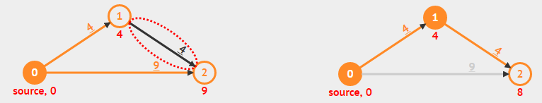

There are three different sources for specifying an input graph:

1. Edit Graph: You can draw, edit, or input any directed weighted graph as the input graph.
2. Example Graphs: You can select from the list of our selected example graphs to get you started. These example graphs have different characteristics.
3. NEW (Oct 24): An NUS student created the following maze/grid-based graph drawing tool that can be quickly used to create a maze/grid graph that can be exported back to this sssp visualization page.

贝尔曼福特的通用算法，虽然有一点慢，但可以解决各种有效的SSSP 问题 (除了一个 ， 我们再以后讨论这个例外)。它还有一个非常简单的伪代码：

for i = 1 to |V|-1 // 这里是 O(V), 所以 O(V×E×1) = O(V×E)
  for each edge(u, v) ∈ E // 这里是 O(E), 例如，通过使用边缘列表
    relax(u, v, w(u, v)) // 这里是 O(1) 

不用多说了，让我们通过点击 BellmanFord(0) 看它在上面的示例图上是如何工作的。（≈30s, 而且现在, 请忽略伪代码底部的附加的循环）。

1. 如果最短路径 p 不是简单路径
2. 那么 p 至少包含一个环 (根据非简单路径的定义)
3. 假设 p 中有一个正权重环 c (如左图的 绿 → 蓝 → 绿)
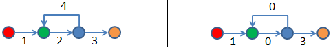
4. 如果我们从 p 中移除 c，那么我们会得到一个比最短路径 p 更短的路径
5. 显然矛盾，所以 p 一定是一个简单路径

6. 就算 c 是一个零权重的环 — 根据我们的定理 1 这是可能的：没有负权重环 (详见右图中的 绿 → 蓝 → 绿)，我们仍然可以从 p 中移除 c 而不增加 p 的权重
7. 总而言之，p 是一个简单路径 (第5点) 或可以被转换成简单路径 (第6点)

或者说，从源顶点 s 到”最远的”（按照最短路径中的边，详见上面的 Bellman-Ford Kill 示例）节点 v 的最短路径 p 最多有 |V|-1 条边。

定理 2: 如果 G = (V, E) 不包含负权重环 , 那么在贝尔曼福特算法终止后，我们将得到 D[v] = δ(s, u), ∀ u ∈ V.

为此, 我们将使用归纳证明法 ，以下是验证的起始点:

考虑从源点 s 到顶点 v_i 的最短路径 p ，其中 v_i 被定义为顶点，从源点 s 到达它的实际最短路径需要 i 次跳 (i 条边) 。回想一下定理 1 ，p 将是简单的路径，因为我们有相同的没有负权重环的假设。

1. 最开始 D[v₀] = δ(s, v₀) = 0, 因为 v₀ 就是源顶点 s
2. 在遍历 E 一遍后，我们有 D[v₁] = δ(s, v₁)
3. 在遍历 E 两遍后，我们有 D[v₂] = δ(s, v₂)
4. ...
5. 在遍历 E k 遍后，我们有 D[v_k] = δ(s, v_k)
6. 如果没有负权重环，最短路径 p 是一个简单路径 (详见定理 1)，所以最后一次遍历是第 |V|-1 次
7. 在 |V|-1 次遍历 E 后，我们有 D[v_|V|-1] = δ(s, v_|V|-1), 不论 E 中边的排序 — 详见上面的 Bellman-Ford Killer 例子

尝试在上面的 'Bellman Ford's Killer' 示例中运行 BellmanFord(0) 。这里有V = 7 个顶点和 E = 6 条边，但是边列表 E 被设置成最差的次序。请注意，在 (V-1)×E = (7-1)*6 = 36 次操作（约40s，耐心等待）之后，贝尔曼福特算法将以正确的答案终止，我们将无法提前终止贝尔曼福特算法。

有的时候，我们面对的实际问题并不是原始问题的普通形式。因此在此电子讲座中，我们会着重于单源最短路径问题的 5 种特殊情况。当我们遇见它们时，我们可以用比 O(V×E) 的贝尔曼福特算法更快的算法解决。这些情况是：

1. 在无权重图中：O(V+E) 的 BFS,
2. 在无负权重图中：O((V+E) log V) 的 戴克斯特拉 (Dijkstra) 算法,
3. 在无负权重的环的图中：O((V+E) log V) 改良版戴克斯特拉 (Dijkstra) 算法,
4. 在树中：O(V+E) 的 DFS/BFS,
5. 在有向无环图中 (DAG): O(V+E) 动态规划 (DP) 算法

O(V+E) 广度优先搜索 (BFS) 算法可以解决有特殊情况的SSSP问题，当输入图是未加权时（所有边都具有单位权重1，在上面的例子 'CP3 4.3' 上尝试 BFS(5)），或者正常数加权（所有有边都具有相同的恒定权重，例如，你可以在上面的例图中用你所选择的任何正恒定权重去更改所有的边的权重）。

当图是未加权 时— 这在现实生活中经常出现— 这种 SSSP 问题可以被视为找到从源点 s 到其它顶点的最小边数的问题。

由快速的 O(V+E) BFS 算法产生的来自源点 s 的BFS的生成树 — 注意符号 ‘+’ — 精确地符合要求。

与贝尔曼福特的 O(V×E) 相比— 注意符号 ‘×’ — 在这个特殊的SSSP中使用 BFS 是明智之举。

与图遍历模块中的标准 BFS 不同，我们需要做简单的修改，使得 BFS 能够解决无权重版本的 SSSP 问题：

1. 首先，我们将布尔数组 visited 改成一个整数数组 D。
2. 在 BFS 开始时，我们不令 visited[u] = false，而是令 D[u] = 1e9 (一个大数字来代表 +∞ 或者 -1 来代表“未访问”状态，但我们不能令 D[0] = 0) ∀u ∈ V\\{s}；然后我们令 D[s] = 0
3. 我们将
   if (visited[v] = 0) { visited[v] = 1 ... } // v 未被访问
   替换成
   if (D[v] = 1e9) { D[v] = D[u]+1 ... } // v 离 u 一步

但是, BFS 很可能在有权重图上运行时产生错误答案，因为 BFS 实际上并不是为解决有权重的SSSP问题而设计的。可能存在这样的情况：采用具有更多边的路径产生的总路径权重总量小于采用具有最小边数量的路径 - 这就是BFS算法的输出。

我们很快会看到戴克斯特拉 (Dijkstra) 算法（2种实现变体）以比一般的贝尔曼福特算法更快的方式解决某些加权SSSP问题。

The O((V+E) log V) Dijkstra's algorithm is the most frequently used SSSP algorithm for typical input: Directed weighted graph that has no negative weight edge, formally: ∀edge(u, v) ∈ E, w(u, v) ≥ 0. Such weighted graph (especially the positive weighted ones) is very common in real life as travelling from one place to another always use positive time unit(s). Try Dijkstra(0) on one of the Example Graphs: CP4 4.16 shown above.

Dijkstra's algorithm maintains a set R(esolved) — other literature use set S(olved) but set S and source vertex s are too close when pronounced — of vertices whose final shortest path weights have been determined. Initially R = {}, empty.

Then, it repeatedly selects vertex u in {V\\R} (can also be written as {V-R}) with the minimum shortest path estimate (the first vertex selected is u = s as initially only D[s] = 0 and the other vertices have D[u] = ∞), adds u to R, and relaxes all outgoing edges of u. Detailed proof of correctness of this Dijkstra's algorithm is usually written in typical Computer Science algorithm textbooks and we replicate it in the next few slides. For a simpler intuitive visual explanation on why this greedy strategy works, see this.

For efficient implementation, this entails the use of a Priority Queue as the shortest path estimates keep changing as more edges are processed. The choice of relaxing edges emanating from vertex with the minimum shortest path estimate first is greedy, i.e., use the "best so far", but we will see later that it can be proven (with loop invariants) that it will ends up with an optimal result — if the graph has no negative weight edge.

在Dijkstra的算法中，每个顶点只会从优先队列（PQ）中提取一次。由于有V个顶点，我们最多会做O(V)次这样的操作。

无论PQ是使用二叉最小堆实现的，还是使用平衡BST如AVL树实现的，ExtractMin()操作都在O(log V)中运行。

因此，这部分是O(V log V)。

每当一个顶点被处理，我们松弛其相邻顶点。总计 E 条边会被处理。

如果当松弛 edge(u, v) 时，我么需要减小 D[v]，我们可以在最小二叉堆中 (较难实现，因为 C++ STL priority_queue/Python heapq/Java PriorityQueue 都不支持此操作) 调用 O(log V) 的 DecreaseKey() 操作；或是简单地在平衡二叉树如AVL树中删除旧项并重新插入新项，这种方法的时间复杂度也为 O(log V)，但更容易实现，因为可以直接调用 C++ STL set/Java TreeSet - 不幸的是Python没有内置支持。

所以，这部分的时间复杂度为 O(E log V)。

To show the correctness of Dijkstra's algorithm on non-negative weighted graph, we need to use loop invariant: a condition which is True at the start of every iteration of the loop.

We want to show:
- Initialization: The loop invariant is true before the first iteration.
- Maintenance: If the loop invariant is true for iteration x, it remains true for iteration x+1.
- Termination: When the algorithm ends, the loop invariant helps the proof of correctness.

Discussion: Formally prove the correctness of Dijkstra's algorithm in class!

当输入图包含至少一个负权重边 —— 不一定是负权重循环 —— 时，Dijkstra的算法可能会产生错误的答案。

尝试在其中一个示例图：CP3 4.18 上点击 Dijkstra(0)。

在执行Dijkstra的算法结束时，顶点4的D[4]值错误，因为算法开始“错误地”认为子路径 0 → 1 → 3 是更好的子路径，权重为 1+2 = 3，因此在调用 relax(3,4,3) 后，D[4] = 6。然而，边 2 → 3 上的负权重 -10 使得另一个子路径 0 → 2 → 3 最终成为更好的子路径，尽管它开始时的路径权重为 10，但在第一条边 0 → 2 后，权重为 10-10 = 0。由于Dijkstra算法的贪婪性质，这个更好的D[3] = 0 永远不会进一步传播，因此D[4]是错误的。

On non-negative weighted graphs, the behavior of Modified Dijkstra's implementation is exactly the same as the Original Dijkstra's so we can use the same time complexity analysis of O((V+E) log V).

PS: We note that when we use the Modified Dijkstra's algorithm, there can be more items (up to E) in the Priority Queue than if we use the Original Dijkstra's algorithm (up to V). However, since O(log E) = O(log V^2) = O(2 log V) = O(log V), we still treat the Priority Queue operations as O(log V).

However, if the graph has at least one negative weight edge, the analysis is harder.

不幸的是, 在一个负权重循环图上运行 ModifiedDijkstra(0) ，如上面的CP3 4.17示例图所示： 将导致无限循环（动画演示很长，但我们将循环数限制为只处理100个边，所以你的网页浏览器不会当机）。

Try ModifiedDijkstra(0) on the extreme corner case above that is very hard to derive without proper understanding of this algorithm and was part of Asia Pacific Informatics Olympiad (APIO) 2013 task set by A/P Halim himself long ago.

The Modified Dijkstra's algorithm will terminate with correct answer, but only after running exponential number of operations (each carefully constructed triangle raises the number of required operations by another power of two). Thus we cannot prematurely terminate Modified Dijkstra's in this worst case input situation.

However, such extreme corner case is rare and thus in practice, Modified Dijkstra's algorithm can be used on directed graphs that have some negative weighted edges as long as the graph has no negative weight cycle reachable from the source vertex s.

O(V) 深度优先搜索 (DFS) 算法可以解决S特殊的SSP 问题，就是当输入图是（加权）树时。

在树中，只有一条独特的无环路径连接两个不同的顶点。因此，将源点 s 链接到任何另一个顶点 u ∈ V 的唯一路径其实上也是最短的路径。例如，在上面的树图上尝试 DFS(0) 。

请注意，对于（加权）树，我们也可以使用BFS。例如，在上面的同一个树图上尝试 BFS(0) 。

讨论：如果输入是一个（加权）树，为什么DFS (以及 BFS) 运行 的是 O(V)而不是 O(V+E) ？

O(V+E) 动态规划 算法可以解决SSSP特殊的问题，就是当输入图是有向无环图（DAG）时 ，我们可以找到至少一个属于这个DAG的拓扑顺序，并根据这个拓扑秩序处理边松弛操作。

例如，在上面示例的DAG上尝试 DP(0) 。 首先，它使用 O(V+E) DFS 或 Graph Traversal 模块中概述的BFS/Kahn 算法.去计算一个（还有其它）可能的拓扑顺序。 比如，假设一个拓扑顺序是 {0,2,1,3,4,5}。然后它松弛该拓扑顺序中列出的外出边。在经过一次 O(V+E) pass 后，我们将得到正确的 D[u] 值， ∀u ∈ V。

在上面显示的修改版的戴克斯特拉杀手示例中， DP(0) 运行得很快，因为尽管具有负权重边，图实际上是一个DAG。并且因此不必担心负权重循环。

但是，DP不适用于任何非DAG，因为非DAG至少包含一个圈，因此在该圈内不能找到拓扑顺序。

用来在 DAG 上求解单源最短路径 (SSSP) 的动态规划算法也被称为 one-pass 贝尔曼福特算法，因为它只用一个拓扑顺序短息（我们知道这是这个DAG的（其中一个）正确顺序）代替最外层的 V-1 圈循环 (我们不知道正确的顺序，所以我们只能重复到达到最大的可能性）。

在上面的实例 DAG 上对比 DP(0) (根据其顶点的拓扑顺序仅松弛 E 边一次）与BellmanFord(0) (以随机顺序松弛 E 边，V-1 次) 。

关于 SSSP 问题，我们还有基于 SSSP 算法的基础解释的许多其他东西。

bellman_ford.cpp/bellman_ford_moore.cpp/dijkstra.cpp
bellman_ford.java/bellman_ford_moore.java/dijkstra.java
bellman_ford.py/bellman_ford_moore.py/dijkstra.py
bellman_ford.ml/bellman_ford_moore.ml/dijkstra.ml

有关此SSSP问题及其各种算法的一些有趣问题，请在 SSSP 培训模块中练习（无需登陆）。

但是，对于注册用户，您应该登陆然后转到 Main Training Page 以正式清除此模块（清除其它先决模块），此类成就将记录在你的账户中。

我们还有一些编程问题，这些问题在某种程度上需要使用正确的SSSP算法：Kattis - hidingplaces 和 Kattis - shortestpath1。

尝试解决它们，然后尝试这个有趣的SSSP问题的更多有趣的变体。

广告：购买竞赛编程教科书以了解更多关于这个有趣问题的信息。