


Pengurutan adalah masalah klasik tentang mengubah urutan elemen-elemen (yang bisa dibandingkan, seperti bilangan bulat, bilangan pecahan, strings, dsb) dari sebuah larik (senarai) ke urutan tertentu (menaik, tidak-menurun (menaik atau datar), menurun, tidak-menaik (menurun atau datar), terurut secara abjad, dsb).
Ada banyak algoritma-algoritma pengurutan, dan masing-masing memiliki kekuatan-kekuatan maupun kekurangan-kekurangan.
Pengurutan biasanya digunakan sebagai masalah pembuka dalam berbagai kelas-kelas Ilmu Komputer untuk menjelaskan berbagai ide-ide algoritma.
Tanpa kehilangan makna umum, kami menggunakan asumsi bahwa kita akan mengurutkan hanya bilangan-bilangan bulat, tidak harus unik, ke dalam urutan tidak-menurun di visualisasi ini. Cobalah klik untuk animasi contoh pengurutan daftar 5 bilangan-bilangan bulat yang tidak beratur (dengan duplikat) diatas.
Remarks: By default, we show e-Lecture Mode for first time (or non logged-in) visitor.
If you are an NUS student and a repeat visitor, please login.
Masalah pengurutan mempunyai berbagai solusi-solusi algoritmik yang menarik dan mencakup banyak ide-ide Ilmu Komputer:
- Strategi pembandingan versus tidak-membandingkan,
- Implementasi iteratif dibandingkan rekursif,
- Paradigma Divide-and-Conquer (Merge Sort atau Quick Sort),
- Analisa kompleksitas waktu Terbaik/Terjelek/Kasus-rata-rata,
- Algoritma-algoritma dengan pengacakan, dsb.
Pro-tip 1: Since you are not logged-in, you may be a first time visitor (or not an NUS student) who are not aware of the following keyboard shortcuts to navigate this e-Lecture mode: [PageDown]/[PageUp] to go to the next/previous slide, respectively, (and if the drop-down box is highlighted, you can also use [→ or ↓/← or ↑] to do the same),and [Esc] to toggle between this e-Lecture mode and exploration mode.
Pada saat sebuah larik bilangan bulat A terurut, banyak masalah-masalah yang berhubungan dengan A menjadi mudah (atau lebih mudah ), silahkan ingat kembali aplikasinya, solusi lebih pelan/sulit dari larik tak terurut, dan solusi lebih cepat/mudah dari larik terurut solutions.
Pro-tip 2: We designed this visualization and this e-Lecture mode to look good on 1366x768 resolution or larger (typical modern laptop resolution in 2021). We recommend using Google Chrome to access VisuAlgo. Go to full screen mode (F11) to enjoy this setup. However, you can use zoom-in (Ctrl +) or zoom-out (Ctrl -) to calibrate this.
Ada dua aksi yang anda dapat lakukan di visualisasi ini.
Pro-tip 3: Other than using the typical media UI at the bottom of the page, you can also control the animation playback using keyboard shortcuts (in Exploration Mode): Spacebar to play/pause/replay the animation, ←/→ to step the animation backwards/forwards, respectively, and -/+ to decrease/increase the animation speed, respectively.
Aksi pertama adalah tentang mendefinisikan masukan anda sendiri, sebuah larik/daftar A yang:
- Betul-betul acak,
- Acak tapi terurut (dalam urutan tidak-menurun atau tidak-menaik),
- Acak tetapi hampir terurut (dalam urutan tidak-menurun atau tidak-menaik),
- Acak dan memiliki banyak duplikat-duplikat (sehingga jangkauan bilangan-bilangan bulatnya kecil), atau
- Didefinisikan oleh anda sendiri.
Dalam mode Eksplorasi, anda dapat bereksperimen dengan berbagai algoritma-algoritma pengurutan yang tersedia di visualisasi ini untuk mengetahui masukan-masukan terbaik dan terjelek untuk algoritma-algoritma tersebut.
Aksi kedua adalah yang terpenting: Jalankan algoritma pengurutan yang sedang aktif dengan meng-klik tombol "Urutkan".
Ingat bahwa anda dapat mengubah algoritma yang aktif dengan meng-klik singkatan di sisi atas dari halaman visualisasi ini.
Lihat visualisasi/animasi dari algoritma pengurutan terpilih disini.
Tanpa kehilangan makna umum, kami hanya menunjukkan bilangan-bilangan bulat didalam visualisasi ini dan tujuan kami adalah untuk mengurutkan mereka dari status awal ke status terurut tidak-menurun. Ingat, tidak-menurun berarti pada umumnya urutan menaik (atau membesar), tetapi karena bisa ada duplikat-duplikat, bisa ada garis datar/sama diantara dua bilangan-bilangan bulat bersisian yang bernilai sama.
Di bagian atas halaman ini, anda akan melihat daftar berbagai algoritma-algoritma pengurutan yang biasanya diajarkan dalam kelas-kelas Ilmu Komputer. Untuk mengaktifkan algoritma tertentu, pilihlah singkatan dari nama algoritma yang bersangkutan sebelum meng-klik "Urutkan".
Untuk memfasilitasi keberagaman, kami akan mengacak algoritma yang aktif setiap kali halaman ini ditampilkan.
Enam algoritma pertama adalah berbasis-pembandingan sedangkan dua terakhir tidak. Kita akan membahas ide ini di pertengahan Kuliah Maya ini.
Tiga algoritma ditengah adalah algoritma pengurutan yang bersifat rekursif sedangkan sisanya biasa diimplementasikan secara iteratif.
Supaya muat di layar, kami menyingkat nama-nama algoritma menjadi tiga karakter saja:
- Algoritma-Algorithma Pengurutan berbasis-pembandingan:
- BUB - Bubble Sort,
- SEL - Selection Sort,
- INS - Insertion Sort,
- MER - Merge Sort (implementasi rekursif),
- QUI - Quick Sort (implementasi rekursif),
- R-Q - Quick Sort Acak (implementasi rekursif).
- Algoritma-Algoritma Pengurutan tidak berbasis-pembandingan:
- COU - Counting Sort,
- RAD - Radix Sort.
Kita akan membahas tiga algoritma-algoritma pengurutan berbasis-pembandingan di beberapa slides berikutnya:
Mereka disebut berbasis-pembandingan karena mereka membandingkan pasangan elemen-elemen dari sebuah larik dan menentukan apakah akan menukar posisi mereka atau tidak.
Ketiga algoritma-algoritma pengurutan ini adalah yang termudah untuk diimplementasikan tetapi juga bukan yang paling efisien, karena mereka berjalan dalam kompleksitas waktu O(N2).
Sebelum kita memulai diskusi berbagai algoritma-algoritma pengurutan, adalah ide bagus untuk membahas dasar-dasar dari analisa algoritma secara asimptotik, sehingga anda dapat mengikuti diskusi-diskusi dari berbagai algoritma-algoritma pengurutan O(N^2), O(N log N), dan spesial O(N) nantinya.
Section ini bisa dilompati jika anda sudah mengetahui topik ini.
Anda butuh untuk sudah mengerti/mengingat hal-hal ini:
-. Logaritma dan Eksponen, misalkan log2(1024) = 10, 210 = 1024
-. Deret Aritmetika, misalkan 1+2+3+4+…+10 = 10*11/2 = 55
-. Deret Geometri, misalkan 1+2+4+8+..+1024 = 1*(1-211)/(1-2) = 2047
-. Fungsi Linear/Kuadratik/Kubik, misalkan f1(x) = x+2, f2(x) = x2+x-1, f3(x) = x3+2x2-x+7
-. Fungsi Langit-Langit, Lantai, dan Absolut, misalkan ceil(3.1) = 4, floor(3.1) = 3, abs(-7) = 7
Analisis algoritma adalah sebuah proses untuk mengevaluasi secara keras sumber daya (waktu dan ruang) yang dibutuhkan oleh sebuah algoritma dan merepresentasikan hasil dari evaluasi tersebut dengan sebuah formula (sederhana).
Kebutuhan waktu/ruang dari sebuah algoritma juga disebut sebagai kompleksitas waktu/ruang dari algoritma tersebut, masing-masing.
Untuk modul ini, kita lebih memfokuskan kepada persyaratan waktu dari berbagai algoritma-algoritma pengurutan.
Kita bisa mengukur waktu perjalanan aktual dari sebuah program dengan menggunakan waktu jam dinding atau dengan memasukkan kode pengukuran-waktu kedalam program kita, misalkan lihat kode yang ditunjukkan didalam SpeedTest.cpp | py | java.
Tetapi, waktu perjalanan aktual tidak berarti banyak ketika membandingan dua algoritma-algoritma karena mereka mungkin ditulis dalam bahasa-bahasa yang berbeda, menggunakan set-set data yang berbeda, atau berjalan pada komputer-komputer yang berbeda.
Daripada mengukur waktu sebenarnya, kita bisa menghitung # dari operasi-operasi (aritmetik, penugasan, pembandingan, dsb). Ini adalah cara untuk mengukur efesiensi karena waktu eksekusi dari sebuah algoritma terkorelasi dengan # operasi-operasi yang dibutuhkannya.
Lihat kode yang ditunjukkan di SpeedTest.cpp | py | java dan komentar-komentarnya (terutama tentang bagaimana mendapatkan nilai final dari variabel counter).
Mengetahu jumlah operasi-operasi (persis) yang dibutuhkan oleh sebuah algoritma, kita bisa menyatakan sesuatu seperti ini: Algoritma X membutuhkan 2n2 + 100n operasi-operasi untuk menyelesaikan masalah dengan ukuran n.
Jika waktu t yang dibutuhkan untuk sebuah operasi diketahu, maka kita bisa menyatakan bahwa algoritma X membutuhkan (2n2 + 100n)t unit-unit waktu untuk menyelesaikan masalah dengan ukuran n.
Tetapi, waktu t tergantung dari faktor-faktor yang disebut sebelumnya, misalkan bahasa-bahasa, kompiler-kompiler, kompleksitas dari operasi tersebut (penjumlahan/pengurangan lebih cepat daripada perkalian/pembagian), dsb.
Oleh karena itu, daripada menghubungkan analisa ke waktu t yang sebenarnya, kita bisa menyatakan bahwa algoritma X membutuhkan waktu yang proporsional terhadap 2n2 + 100n untuk menyelesaikan masalah dengan ukuran n.
Analisa Asimtotik adalah sebuah analisa algoritma-algoritma yang berfokus pada penganalisaan masalah-masalah dengan ukuran masukan n yang besar, memikirkan hanya term tertinggi saja dari formula, dan mengabaikan koefisien dari term tertinggi.
Kita memilih term tertinggi karena term-term yang lebih kecil berkontribusi lebih sedikit kepada biaya total saat ukuran masukan bertumbuh besar, misalkan untuk f(n) = 2n2 + 100n, kita punya:
f(1000) = 2*10002 + 100*1000 = 2.1M, versus
f(100000) = 2*1000002 + 100*100000 = 20010M.
(sadari bahwa term yang lebih kecil 100n memiliki kontribusi yang lebih kecil).
Misalkan dua algoritma-algoritma memiliki 2n2 dan 30n2 sebagai term-term tertinggi.
Meskipun waktu sebenarnya akan berbeda karena konstanta-konstanta yang berbeda, laju-laju pertumbuhan dari waktu eksekusi adalah sama.
Dibandingkan dengan algoritma lain dengan term tertinggi n3, perbedaan dari laju pertumbuhan adalah faktor yang jauh lebih dominan.
Maka, kita bisa melepaskan koefisien dari term tertinggi ketika mempelajari kompleksitas algoritma.
Jika algoritma A membutuhkan waktu proporsional terhadap f(n), kita bilang bahwa algoritma A berada dalam order f(n).
Kita menulis bahwa algoritma A mempunyai kompleksitas waktu O(f(n)), dimana f(n) adalah fungsi laju pertumbuhan untuk algoritma A.
Secara matematis, sebuah algoritma adalah O(f(n)) jika ada sebuah konstanta k dan sebuah bilangan bulat positif n0 sehingga algoritma A membutuhkan tidak lebih dari k*f(n) unit-unit waktu untuk menyelesaikan sebuah masalah dengan ukuran n ≥ n0, yaitu, jika ukuran masalah lebih besari dari n0, algoritma A (selalu) dibatasi dari atas oleh formula sederhana k*f(n) ini.
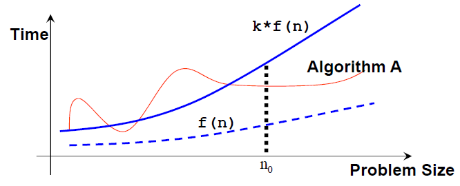
Catat bahwa: n0 dan k tidak unik dan bisa ada beberapa banyak f(n) valid yang memungkinkan.
Dalam analisa asimtotik, sebuah formula bisa disederhanakan menjadi sebuah term tunggal dengan koefisien 1.
Term tersebut disebut sebagai term pertumbuhan (tingkat pertumbuhan, urutan pertumbuhan, urutan besar).
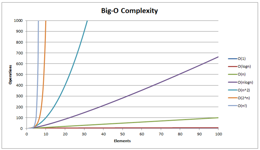
Term-term pertumbuhan yang paling umum dapat diurutkan dari yang paling cepat ke paling lambat sebagai berikut:
O(1)/waktu konstan < O(log n)/waktu logaritmik < O(n)/waktu linear <
O(n log n)/waktu kuasilinear < O(n2)/waktu kuadratik < O(n3)/waktu kubik <
O(2n)/waktu eksponensial < O(n!)/waktu juga-eksponensial < ∞ (misalkan, perulangan tak berakhir).
Catat bahwa ada beberapa kompleksitas-kompleksitas waktu yang umum lainnya yang tidak ditunjukkan (lihat juga visualisasi di slide berikutnya)).
Kita akan melihat tiga laju-laju pertumbuhan yang berbeda O(n2), O(n log n), dan O(n) sepanjang sisa dari modul pengurutan ini.
- Membandingkan pasangan yang bersebelahan (a, b),
- Menukar pasangan tersebut bila tidak pada urutan yang seharusnya (dalam kasus ini, ketika a > b),
- Ulangi Langkah 1 dan 2 hingga kita sampai di akhir larik
(pasangan terakhir adalah elemen ke (N-2) dan (N-1) karena kita menggunakan indeks basis-0), - Pada saat ini, elemen terbesar akan terletak pada posisi terakhir.
Kita lalu mengurangi N dengan 1 dan kembali ke Langkah 1 sampai kita mendapat N = 1.
Tanpa basa-basi lagi, mari coba pada larik contoh kecil [29, 10, 14, 37, 14].
Anda akan melihat animasi 'seperti-gelembung' jika anda membayangkan elemen-elemen yang besar 'menggelembung keatas' (atau sebenarnya 'bergerak ke sisi kanan dari larik').
method bubbleSort(array A, integer N) // versi standar
  untuk tiap R dari N-1 turun ke 1 // ulangi N-1 kali
    untuk tiap indeks i dalam [0..R-1] // indeks tak terurut, O(N)
      jika A[i] > A[i+1] // tidak dalam urutan tidak-menurun
        tukar(a[i], a[i+1]) // tukar dalam O(1)
Pembandingan dan penukaran membutuhkan waktu yang dibatasi oleh sebuah konstanta, mari sebut saja dengan c. Lalu, ada dua perulangan (loop) yang bertingkat (nested) dalam Bubble Sort standar. Perulangan (loop) luar berjalan tepat sebanyak N iterasi. Tetapi pengulangan (loop) dalam menjadi sedikit lebih pendek pada setiap iterasi:
- Saat R=N-1, (N−1) iterasi (dari pembandingan-pembandingan dan kemungkinan pertukaran-pertukaran),
- Saat R=N-2, (N−2) iterasi,
- Saat R=1, 1 iterasi (lalu selesai).
Sehingga, jumlah total dari iterasi = (N−1)+(N−2)+...+1+0 = N*(N−1)/2 (penurunan)
Waktu total adalah = c*N*(N−1)/2 = O(N^2)
Lihatlah kode dari SortingDemo.cpp | py | java.
Bubble Sort sebenarnya tidak efisien dengan kompleksitas waktu O(N^2). Bayangkan jika kita memiliki N = 105 angka-angka. Meskipun komputer kita sangat cepat dan dapat menghitung 108 operasi-operasi dalam 1 detik, Bubble Sort akan membutuhkan sekitar 100 detik untuk menyelesaikan tugas ini.
Tetapi, Bubble Sort dapat dihentikan lebih awal, misalkan pada contoh kecil yang telah terurut menaik diatas [3, 6, 11, 25, 39], dapat dihentikan dalam waktu O(N).
Idenya mudah: Jika kita melalui perulangan dalam (inner loop) tanpa melakukan pertukaran sama sekali, itu berarti bahwa larik tersebut sudah terurut dan kita dapat menghentikan Bubble Sort pada saat itu.
Diskusi: Meskipun ide tersebut membuat Bubble Sort berjalan lebih cepat dalam kasus-kasus umum, ide ini tidak mengubah kompleksitas waktu O(N^2) dari Bubble Sort... Kenapa?
The content of this interesting slide (the answer of the usually intriguing discussion point from the earlier slide) is hidden and only available for legitimate CS lecturer worldwide. This mechanism is used in the various flipped classrooms in NUS.
If you are really a CS lecturer (or an IT teacher) (outside of NUS) and are interested to know the answers, please drop an email to stevenhalim at gmail dot com (show your University staff profile/relevant proof to Steven) for Steven to manually activate this CS lecturer-only feature for you.
FAQ: This feature will NOT be given to anyone else who is not a CS lecturer.
Diberikan sebuah larik berisi N elemen dan L = 0, Selection Sort akan:
- Menemukan posisi X dari elemen terkecil dalam interval [L...N-1],
- Tukar item ke-X dengan item ke-L,
- Naikkan batas bawah L sebesar 1 dan kembail ke Langkah 1 sampai L = N-2.
Mari coba pada larik contoh kecil yang sama [29, 10, 14, 37, 13].
Tanpa kehilangan makna umum, kita juga dapat mengimplementasikan Selection Sort secara terbalik:
Temukan posisi dari elemen terbesar Y dan tukar dengan elemen terakhir.
method selectionSort(array A[], integer N)
  untuk tiap L dalam [0..N-2] // O(N)
    misalkan X merupakan indeks dari elemen minimum dalam A[L..N-1] // O(N)
    tukar(A[X], A[L]) // O(1), X may be equal to L (no actual swap)
Total: O(N2) — Lebih tepatnya, ini mirip dengan analisa Bubble Sort.
Lihatlah kode dari SortingDemo.cpp | py | java.
Quiz: How many (real) swaps are required to sort [29, 10, 14, 37, 13] by Selection Sort?
Insertion Sort mirip dengan bagaimana kebanyakan orang menyusun kartu poker di tangan. 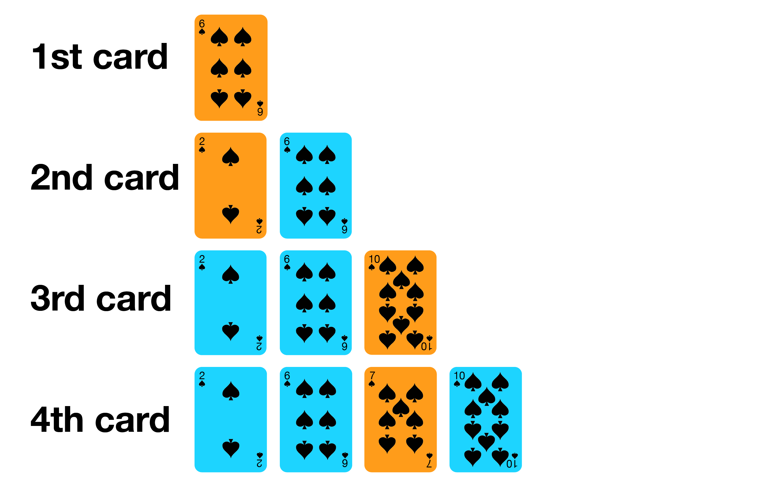
- Mulai dengan satu kartu di tangan,
- Pilih kartu berikutnya dan masukkan ke dalam posisi yang benar,
- Ulang langkah tersebut untuk seluruh kartu.
method insertionSort(array A[], integer N)
  for i in [1..N-1] // O(N)
    let X be A[i] // item selanjutnya untuk dimasukkan dalam A[0..i-1]
    for j from i-1 down to 0 // loop ini bisa cepat atau lambat
      if A[j] > X
        A[j+1] = A[j] // buat tempat untuk X
      else
        break
    A[j+1] = X // masukkan X pada indeks j+1
Lihatlah kode dari SortingDemo.cpp | py | java.
Perulangan luar (outer loop) dijalankan N−1 kali, sepertinya ini cukup jelas.
Tetapi berapa kali perulangan dalam (inner loop) dilakukan tergantung pada masukan:
- Dalam kasus terbaik, larik sudah terurut menaik dan (a[j] > X) selalu salah
Sehingga tidak ada pergeseran data yang terjadi dan perulangan dalam (inner loop) berjalan dalam O(1), - Dalam kasus terjelek, larik terurut terbalik (menurun) dan (a[j] > X) selalu benar
Pemasukkan (insertion) selalu terjadi di depan larik dan perulangan dalam (inner loop) berjalan dalam O(N).
Sehingga, waktu terbaik adalah O(N × 1) = O(N) dan waktu terburuk adalah O(N × N) = O(N2).
Quiz: What is the complexity of Insertion Sort on any input array?
Tanya instruktor anda bila anda tidak mengerti tentang hal ini atau baca catatan yang sejenis di slide ini.
Kita akan membahas dua (dan setengah) algoritma-algoritma berbasis-pembandingan segera:
- Merge Sort,
- Quick Sort dan versi acaknya (yang hanya memiliki satu perubahan).
Algoritma-algoritma pengurutan ini biasanya diimplementasikan secara rekursif, menggunakan paradigma pemecahan masalah Divide and Conquer, dan berjalan dalam waktu O(N log N) untuk Merge Sort dan O(N log N) secara ekspektasi untuk Quick Sort Acak.
PS: Versi tidak-acak dari Quick Sort sayangnya berjalan dalam waktu O(N2).
Diberikan sebuah larik berisi N elemen, Merge Sort akan:
- Menggabungkan tiap pasang elemen (yang secara default terurut) menjadi larik-larik berukuran 2 elemen,
- Menggabungkan tiap pasang larik-larik tersebut menjadi larik-larik berukuran 4 elemen, Ulangi proses ini...,
- Langkah terakhir: Menggabungkan 2 larik-larik yang sudah terurut dengan jumlah N/2 elemen (untuk memudahkan diskusi, kita berasumsi bahwa N genap) untuk mendapatkan larik yang terurut penuh dengan jumlah N elemen.
Ini hanyalah ide general dan kita membutuhkan beberapa detail tambahan sebelum kita bisa membahas bentuk sebenarnya dari Merge Sort.
Kita akan membahas dengan detil algoritma Merge Sort ini dengan pertama-tama membahas sub-rutin terpentingnya: Proses penggabungan (merge) dalam O(N).
Diberikan dua larik yang sudah terurut, A dan B, dengan ukuran N1 dan N2, kita dapat dengan efisien menggabungkan mereka mejadi satu larik terurut yang lebih besar dengan ukuran N = N1+N2, dalam waktu O(N).
Ini dapat diraih dengan cara membandingkan elemen terdepan dari kedua larik dan mengambil yang terkecil dari dua itu setiap waktu. Tetapi, sub-rutin merge yang sederhana tapi cepat O(N) ini akan membutuhkan larik tambahan untuk melakukan proses penggabungan ini dengan benar.
method merge(array A, integer low, integer mid, integer high)
  // sublarik1 = a[low..mid], sublarik2 = a[mid+1..high], keduanya terurut
  int N = high-low+1
  create array B of size N // diskusi: kenapa kita perlu larik temp b?
  int left = low, right = mid+1, bIdx = 0
  while (left <= mid && right <= high) // merge
    if (A[left] <= A[right])
      B[bIdx++] = A[left++]
    else
      B[bIdx++] = A[right++]
  while (left <= mid)
    B[bIdx++] = A[left++] // sisanya, jika ada
  while (right <= high)
    B[bIdx++] = A[right++] // sisanya, jika ada
  for (int k = 0; k < N; ++k)
    A[low+k] = B[k]; // salin kembali
Cobalah pada larik contoh [1, 5, 19, 20, 2, 11, 15, 17] yang sebagian pertamanya telah terurut [1, 5, 19, 20] dan sebagian keduanya juga telah terurut [2, 11, 15, 17]. Fokus kepada penggabungan terakhir dari algoritma Merge Sort.
Sebelum kita lanjutkan, mari berbicara tentang Divide and Conquer (disingkat sebagai D&C), sebuah paradigma pemecahan masalah yang kuat.
Algoritma Divide and Conquer menyelesaikan (sejenis) masalah — seperti masalah pengurutan kita — dalam beberapa langkah-langkah berikut:
- Langkah Divide: Membagi masalah yang asli dan besar menjadi masalah-masalah yang lebih kecil dan secara rekursif menyelesaikan masalah-masalah yang lebih kecil tersebut,
- Langkah Conquer: Gabungkan hasil-hasil dari masalah-masalah yang lebih kecil tersebut untuk menghasilkan hasil dari masalah yang asli dan besar.
Merge Sort adalah algoritma pengurutan bersifat Divide and Conquer.
Langkah pembagian (divide) mudah saja: Bagi larik yang sekarang menjadi dua bagian (sama besar jika N genap atau satu sisi satu elemen sedikit lebih besar jika N ganjil) dan lalu secara rekursif mengurutkan kedua bagian tersebut.
Langkah penaklukkan (conquer) adalah langkah yang melakukan usaha terbesar: Gabungkan dua bagian (yang sudah terurut) untuk membentuk larik yang terurut, menggunakan sub-rutin penggabungan (merge) yang dibahas sebelumnya.
method mergeSort(array A, integer low, integer high)
  // larik yang akan diurutkan adalah A[low..high]
  if (low < high) // kasus dasar: low >= high (0 or 1 item)
    int mid = (low+high) / 2
    mergeSort(a, low  , mid ) // bagi jadi dua bagian
    mergeSort(a, mid+1, high) // lalu urutkan secara rekursif
    merge(a, low, mid, high) // kuasai: sub-rutin merge
Lihatlah kode dari SortingDemo.cpp | py | java.
Dibandingkan dengan apa yang biasanya ditampilkan di banyak buku-buku teks Ilmu Komputer yang dicetak (karena buku-buku sifatnya statis), eksekusi sebenarnya dari Merge Sort tidak membagi kedua sub-larik level demi level, tetapi Merge Sort akan secara rekursif mengurutkan sub-larik kiri terlebih dahulu sebelum mengurutkan sub-larik kanan.
Lebih detailnya, menjalankan pada larik contoh [7, 2, 6, 3, 8, 4, 5], Merge Sort akan merekursi ke [7, 2, 6, 3], lalu [7, 2], lalu [7] (sebuah elemen tunggal, yang sudah terurut secara default), kembali, rekursi ke [2] (terurut), kembali, lalu menggabungkan [7, 2] menjadi [2, 7], sebelum Merge Sort memproses [6, 3] dan selanjutnya.
Dalam Merge Sort, usaha terbanyak dilakukan dalam langkah conquer/merge karena langkah divide sebenarnya tidak melakukan apa-apa (dianggap O(1)).
Ketika kita memanggil merge(a, low, mid, high), kita memproses k = (high-low+1) elemen.
Akan ada paling banyak k-1 pembandingan.
Ada k perpindahan dari larik asli a ke larik temporer b dan k perpindahan lainnya untuk menyalin balik.
Secara total, jumlah operasi dalam operasi sub-rutin merge adalah < 3k-1 = O(k).
Pertanyaan penting berikutnya adalah berapa kali sub-rutin merge ini dipanggil?
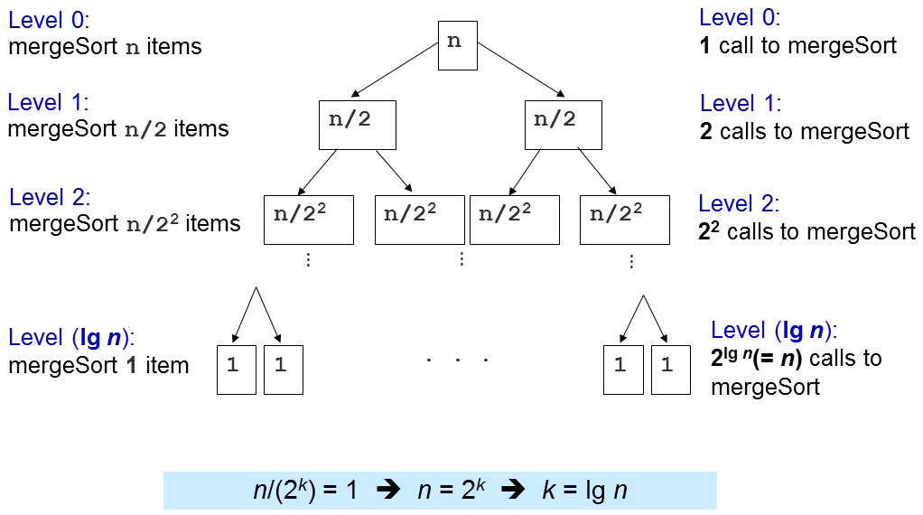
Level 1: 2^0=1 panggilan kepada merge() dengan N/2^1 elemen masing-masing, O(2^0 x 2 x N/2^1) = O(N)
Level 2: 2^1=2 panggilan kepada merge() dengan N/2^2 elemen masing-masing, O(2^1 x 2 x N/2^2) = O(N)
Level 3: 2^2=4 panggilan kepada merge() dengan N/2^3 elemen masing-masing, O(2^2 x 2 x N/2^3) = O(N)
...
Level (log N): 2^(log N-1) (atau N/2) panggilan kepada merge() dengan N/2^log N (or 1) elemen masing-masing, O(N)
Ada log N level dan di setiap level, kita melakukan usaha sebesar O(N), sehingga kompleksitas waktu seluruhnya adalah O(N log N). Nanti, kita akan melihat bahwa ini adalah algoritma pengurutan (berbasis-pembandingan) yang sudah optimal, atau dengan kata lain, kita tidak bisa membuat algoritma lebih baik dari Merge Sort ini.
Bagian bagus dari Merge Sort yang paling penting adalah garansi performa O(N log N), tidak tergantung pada urutan asli dari masukan. Dengan kata lain, tidak ada kasus tes yang bisa membuat Merge Sort berjalan lebih lambat dari O(N log N) untuk segala larik dengan N elemen.
Merge Sort sangat cocok untuk mengurutkan masukan yang sangat besar karena O(N log N) bertumbuh jauh lebih lambat dari algoritma-algoritma pengurutan yang membutuhkan waktu O(N2) seperti yang dibahas sebelumnya.
Tetapi ada juga beberapa bagian yang tidak bagus dari Merge Sort. Pertama, sebenarnya tidak mudah untuk mengimplementasikan Merge Sort dari awal (tetapi sebenarnya kita tidak perlu melakukannya). Kedua, Merge Sort membutuhkan tempat tambahan sebesar O(N) dalam proses penggabungan, sehingga tidak efisien secara memori dan tidak di-tempat. Ngomong-ngomong, bila anda tertarik untuk melihat apa yang sudah dilakukan untuk mengatasi bagian yang tidak bagus dari Merge Sort (klasik) ini, anda bisa membaca ini
Merge Sort juga adalah algoritma pengurutan yang stabil. Diskusi: Kenapa?
The content of this interesting slide (the answer of the usually intriguing discussion point from the earlier slide) is hidden and only available for legitimate CS lecturer worldwide. This mechanism is used in the various flipped classrooms in NUS.
If you are really a CS lecturer (or an IT teacher) (outside of NUS) and are interested to know the answers, please drop an email to stevenhalim at gmail dot com (show your University staff profile/relevant proof to Steven) for Steven to manually activate this CS lecturer-only feature for you.
FAQ: This feature will NOT be given to anyone else who is not a CS lecturer.
Quick Sort adalah algoritma pengurutan lain yang juga berbasis Divide and Conquer (satu lagi yang telah dibahas di Kuliah Maya ini adalah Merge Sort).
Kita akan melihat bahwa versi deterministik, tidak acak dari Quick Sort bisa memiliki kompleksitas waktu yang jelek, yaitu O(N2) pada masukan jahat (adversary) sebelum kita melanjutkan pembahasan dengan versi acak yang lebih bisa dipakai nantinya.
Langkah Divide: Pilih elemen p (dinamai sebagai pivot)
Lalu partisi (partition) elemen-elemen A[i..j] menjadi tiga bagian: A[i..m-1], A[m], dan A[m+1..j].
A[i..m-1] (kemungkinan kosong) berisi elemen-elemen yang lebih kecil dari p.
A[m] adalah pivot p, indeks m adalah posisi p yang benar didalam larik terurut a nantinya.
A[m+1..j] (kemungkinan kosong) berisi elemen-elemen yang lebih besar atau sama dengan p.
Lalu, urutkan kedua bagian ini secara rekursif.
Langkah Conquer: Jangan kaget... Kita tidak melakukan apa-apa :O!
Jika anda membandingkan ini dengan Merge Sort, anda akan melihat bahwa langkah-langkah D&C dari Quick Sort terbalik total dengan Merge Sort.
Kita akan membahas dengan detil algoritma Quick Sort ini dengan pertama-tama membahas sub-rutin terpentingnya: O(N) partition.
Untuk mempartisi A[i..j], kita pertama-tama memilih A[i] sebagai pivot p.
Elemen-elemen sisanya (yaitu A[i+1..j]) terbagi jadi 3 wilayah:
- S1 = A[i+1..m] dimana elemen-elemennya < p,
- S2 = A[m+1..k-1] dimana elemen-elemennya ≥ p, dan
- Tidak diketahui = A[k..j], dimana elemen-elemennya belum dimasukkan ke S1 atau S2.
Diskusi: Kenapa kita memilih p = A[i]? Apakah ada pilihan-pilihan yang lain?
Diskusi yang lebih susah: Jika A[k] == p, apakah kita letakkan pada S1 atau S2?
The content of this interesting slide (the answer of the usually intriguing discussion point from the earlier slide) is hidden and only available for legitimate CS lecturer worldwide. This mechanism is used in the various flipped classrooms in NUS.
If you are really a CS lecturer (or an IT teacher) (outside of NUS) and are interested to know the answers, please drop an email to stevenhalim at gmail dot com (show your University staff profile/relevant proof to Steven) for Steven to manually activate this CS lecturer-only feature for you.
FAQ: This feature will NOT be given to anyone else who is not a CS lecturer.
Pada awalnya, region S1 dan S2 dua-duanya kosong, yaitu semua elemen kecuali pivot p yang terpilih berada dalam region yang tidak diketahui.
Lalu, untuk setiap elemen A[k] di region yang tidak diketahui, kita membandingkan A[k] dengan p dan memutuskan satu dari tiga kasus berikut:
- Jika A[k] > p, taruh A[k] di S2,
- Jika A[k] < p, taruh A[k] di S1,
- Jika A[k] == p, lempar sebuah koin dan taruh A[k] ke S1/S2 jika jatuh kepala/ekor, masing-masing.
Ketiga kasus-kasus ini akan dijelaskan lebih detil di dua slide berikutnya.
Pada akhirnya, kita menukar A[i] dan A[m] untuk menaruh pivot p tepat diantara S1 dan S2.
![Case when a[k] ≥ p, increment k, extend S2 by 1 item](https://visualgo.net/img/partition1.png)
![Case when a[k] < p, increment m, swap a[k] with a[m], increment k, extend S1 by 1 item](https://visualgo.net/img/partition2.png)
int partition(array A, integer i, integer j)
  int p = a[i] // p sebagai pivot
  int m = i // S1 dan S2 pada mulanya kosong
  for (int k = i+1; k <= j; ++k) // jelajah bagian baru
    if ((A[k] < p) || ((A[k] == p) && (rand()%2 == 0)))  { // kasus 2+3
      ++m
      swap(A[k], A[m]) // tukar kedua indeks tersebut
    // kita tidak melakukan apa-apa pada kasus 1: a[k] > p
  swap(A[i], A[m]) // langkah terakhir, tukar pivot dengan a[m]
  return m // kembalikan indeks pivot
method quickSort(array A, integer low, integer high)
  if (low < high)
    int m = partition(a, low, high) // O(N)
    // A[low..high] ~> A[low..m–1], pivot, A[m+1..high]
    quickSort(A, low, m-1); // urutkan sublarik kiri secara rekursif
    // A[m] = pivot sudah terurut setelah partisi
    quickSort(A, m+1, high); // lalu urutkan sublarik kanan
Lihatlah kode dari SortingDemo.cpp | py | java.
Coba pada larik contoh [27, 38, 12, 39, 29, 16]. Kita akan bahas langkah pertama dari partition sebagai berikut:
Kita set p = A[0] = 27.
Kita set A[1] = 38 sebagai bagian S2 jadi S1 = {} dan S2 = {38}.
Kita tukar A[1] = 38 dengan A[2] = 12 jadi S1 = {12} dan S2 = {38}.
Kita set A[3] = 39 dan juga A[4] = 29 berikutnya sebagai bagian S2 jadi S1 = {12} dan S2 = {38,39,29}.
Kita tukar A[2] = 38 dengan A[5] = 16 jadi S1 = {12,16} dan S2 = {39,29,38}.
Kita tukar p = A[0] = 27 dengan A[2] = 16 jadi S1 = {16,12}, p = {27}, dan S2 = {39,29,38}.
Setelah ini, A[2] = 27 dijamin terurut sekarang dan Quick Sort akan mengurutkan secara rekursif sisi kiri A[0..1] duluan dan nanti mengurutkan secara rekursif sisi kanan A[3..5].
Pertama-tama, kita analisa biaya satu pemanggilan partition.
Didalam partition(A, i, j), hanya ada satu for-loop yang diulang (j-i) kali. Karena j bisa sebesar N-1 dan i bisa sekecil 0, maka kompleksitas waktu dari partition adalah O(N).
Mirip dengan analisa Merge Sort, kompleksitas waktu dari Quick Sort tergantung seberapa banyak partition(A, i, j) dipanggil.
Ketika larik A sudah dalam urutan menaik, misalkan A = [5, 18, 23, 39, 44, 50}, akan mengatur p = A[0] = 5, dan akan mengembalikan m = 0, oleh karena itu membuat region S1 kosong dan region S2: Semuanya kecuali pivot (N-1 elemen).
Pada skenario terjelek tersebut, inilah yang terjadi:
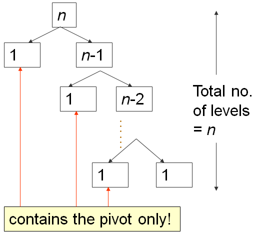
Partisi pertama membutuhkan waktu O(N), membagi A menjadi 0, 1, N-1 elemen-elemen, lalu rekursi ke-kanan.
Yang kedua membutuhkan waktu O(N-1), membagi A menjadi 0, 1, N-2 elemen-elemen, lalu rekursi ke-kanan lagi.
...
Sampai yang terakhir, uartisi ke N membagi A menjadi 0, 1, 1 elemen, dan rekursi Quick Sort berhenti.
Ini adalah pola klasik N+(N-1)+(N-2)+...+1, yang disederhanakan sebagai O(N2), analisa yang mirip dengan yang di slide analisa Bubble Sort ini...
Skenario terbaik dari Quick Sort terjadi ketika partition selalu membagi larik menjadi dua bagian yang sama besar, seperti Merge Sort.
Ketika itu terjadi, kedalaman rekursi hanyalah O(log N).
Karena setiap level membutuhkan O(N) pembandingan, kompleksitas waktu adalah O(N log N).
Coba di contoh larik masukan yang telah dipersiapkan secara khusus [4, 1, 3, 2, 6, 5, 7].
Pada prakteknya, hal ini jarang terjadi, sehingga kita harus memikirkan cara yang lebih baik: Quick Sort Acak.
Sama seperti Quick Sort tetapi sebelum menjalankan algoritma partisi, algoritma ini secara acak memilih sebuah pivot diantara A[i..j] dibandingkan dengan selalu memilih A[i] (atau indeks tetap lainnya diantara [i..j]) secara deterministik.
Latihan kecil: Implementasikan ide diatas pada implementasi yang ditunjukkan di slide ini!
Coba pada larik yang besar dan agak acak A = [3,44,38,5,47,15,36,26,27,2,46,4,19,50,48] terasa cepat.
Akan dibutuhkan kuliah sekitar 1 jam untuk menjelaskan dengan baik kenapa versi acak dari Quick Sort mempunyai kompleksitas waktu yang diharapkan O(N log N) pada larik masukan apapun dengan N elemen.
Dalam Kuliah Maya ini, kita akan berasumsi bahwa ini benar.
Jika anda membutuhkan penjelasan non formal: Bayangkan bahwa versi acak dari Quick Sort yang mengacak pemilihan pivot, kita tidak akan selalu mendapat pembagian yang sangat jelek yaitu 0 (kosong), 1 (pivot), dan N-1 elemen lainnya. Kombinasi dari beruntung (setengah-pivot-setengah), kira-kira beruntung, kira-kira tidak beruntung, dan sangat tidak beruntung (kosong, pivot, sisanya) menghasilkan kompleksitas waktu rata-rata O(N log N).
Diskusi: Untuk implementasi dari Partisi, apa yang terjadi jika A[k] == p, kita selalu menaruh A[k] pada salah satu sisi (S1 atau S2) secara deterministik?
The content of this interesting slide (the answer of the usually intriguing discussion point from the earlier slide) is hidden and only available for legitimate CS lecturer worldwide. This mechanism is used in the various flipped classrooms in NUS.
If you are really a CS lecturer (or an IT teacher) (outside of NUS) and are interested to know the answers, please drop an email to stevenhalim at gmail dot com (show your University staff profile/relevant proof to Steven) for Steven to manually activate this CS lecturer-only feature for you.
FAQ: This feature will NOT be given to anyone else who is not a CS lecturer.
Kita akan membahas dua algoritma-algoritma pengurutan yang tidak berbasis-pembandingan di beberapa slide berikut ini:
Algoritma-algoritma pengurutan ini bisa lebih cepat dari batas bawah algoritma pengurutan berbasis-pembandingan yaitu Ω(N log N) karena mereka tidak membandingkan elemen-elemen dari larik.
Sudah diketahui (tapi tidak dibuktikan di Kuliah Maya ini karena akan membutuhkan 1 jam kuliah lagi) bahwa semua algortima pengurutan berbasis-pembandingan mempunyai kompleksitas waktu batas bawah sebesar Ω(N log N).
Jadi, algoritma pengurutan berbasis-pembandingan apapun dengan kompleksitas terjelek O(N log N), seperti Merge Sort sebenarnya algoritma yang sudah optimal, kita tidak bisa berbuat lebih baik dari itu.
Tetapi, kita dapat mendapatkan algoritma pengurutan yang lebih cepat — yaitu dalam O(N) — jika ada beberapa asumsi-asumsi dari larik masukan sehingga kita dapat menghindari pembandingan dari elemen-elemen untuk menentukan urutan.
Asumsi: Jika elemen-elemen yang akan diurutkan adalah bilangan-bilangan bulat dengan range kecil, kita dapat menghitung frekuensi dari setiap bialngan bulat (dalam range kecil tersebut) dan lalu mengecek range kecil tersebut untuk mengeluarkan elemen-elemen tersebut dalam urutan terurut.
Coba pada larik contoh diatas dimana semua bilangan-bilangan bulat berada dalam [1..9], sehingga kita hanya perlu menghitung berapa kali bilangan 1 muncul, bilangan 2 muncul, ..., bilangan 9 muncul, dan lalu mengecek 1 sampai 9 untuk mencetak x kopi dari bilangan y jika frekuensi[y] = x.
Kompleksitas waktunya adalah O(N) untuk menghitung frekuensi-frekuensi dan O(N+k) untuk mencetak keluaran dalam urutan terurut di mana k adalah range dari bilangan-bilangan bulat masukan, yang adalah 9-1+1 = 9 dalam contoh ini. Kompleksitas waktu dari Counting Sort menjadi O(N+k), yang adalah O(N) jika k kecil.
Kita tidak bisa melakukan bagian perhitungan dari Counting Sort ketika k cukup besar karena keterbatasan memori, karena kita harus menyimpan frekuensi-frekuensi dari k bilangan-bilangan bulat tersebut.
Catatan: Versi Counting Sort ini tidak stabil, karena algoritma versi ini tidak mengingatkan urutan masukan dari bilangan duplikat. Versi yang diberikan dalam CLRS stabil, tapi sedikit lebih rumit dari formulasi kami sekarang.
Asumsi: Jika elemen-elemen yang akan diurutkan adalah bilangan-bilangan bulat dengan range besar tetapi sedikit jumlah digit, kita dapat menggabungkan ide Counting Sort dengan Radix Sort untuk mencapai kompleksitas waktu linear.
Dalam Radix Sort, kita memperlakukan setiap elemen yang akan diurutkan sebagai string dengan w digit (kita tambahkan bilangan-bilangan bulat yang mempunyai kurang dari w digit dengan angka nol pembuka jika diperlukan).
Dari digit yang paling tidak signifikan (yang paling kanan) ke digit yang paling signifikan (yang paling kiri), kita melakukan satu pass ke semua N elemen-elemen dan menaruh mereka sesuai dengan digit aktif ke 10 Antrean (Queues) (satu untuk setiap digit [0..9]), yang seperti Counting Sort termodifikasi karena yang ini menjaga stabilitas. (ingat, versi Counting Sort yang ditunjukkan di slide sebelumnya bukanlah pengurutan stabil). Lalu kita menggabungkan kembali group-group tersebut untuk iterasi selanjutnya.
Coba pada larik masukan contoh diatas untuk penjelasan yang lebih baik.
Catat bahwa kita hanya melakukan O(w × (N+k)) iterasi. Di contoh ini, w = 4 dan k = 10.
Sekarang, setelah kita mendiskusikan Radix Sort, haruskah kita menggunakannya untuk setiap situasi pengurutan?
The content of this interesting slide (the answer of the usually intriguing discussion point from the earlier slide) is hidden and only available for legitimate CS lecturer worldwide. This mechanism is used in the various flipped classrooms in NUS.
If you are really a CS lecturer (or an IT teacher) (outside of NUS) and are interested to know the answers, please drop an email to stevenhalim at gmail dot com (show your University staff profile/relevant proof to Steven) for Steven to manually activate this CS lecturer-only feature for you.
FAQ: This feature will NOT be given to anyone else who is not a CS lecturer.
Ada beberapa properti-properti lain yang bisa digunakan untuk membedakan algoritma-algoritma pengurutan lebih dari sekedar apakah mereka berbasis-pembandingan atau tidak, rekursif atau iteratif.
Dalam bagian ini, kita akan membahas tentang di-tempat dibandingkan dengan tidak di-tempat, stabil dibandingkan dengan tidak stabil, dan performa caching dari berbagai algoritma-algoritma pengurutan.
Sebuah algoritma pengurutan dikatakan sebagai pengurutan di-tempat jika algoritma tersebut hanya membutuhkan sejumlah ruang konstan (yaitu O(1)) selama proses pengurutan. Dengan kata lain, beberapa (konstan) variable-variable ekstra diperbolehkan tetapi kita tidak diperbolehkan untuk menggunakan variable-variable yang mempunyai ukuran tergantung kepada ukuran masukan N.
Merge Sort (versi klasik), karena sub-rutin merge nya membutuhkan larik temporer tambahan dengan ukuran N, tidak di-tempat.
Diskusi: Bagaimana dengan Bubble Sort, Selection Sort, Insertion Sort, Quick Sort (acak maupun tidak), Counting Sort, dan Radix Sort. Yang mana saja yang di-tempat?
Sebuah algoritma pengurutan dikatakan stabil bila urutan relatif dari elemen-elemen dengan nilai yang sama tetap terpelihara oleh algoritma tersebut setelah pengurutan dilakukan.
Contoh aplikasi dari pengurutan stabil: Asumsikan bahwa kita memiliki nama-nama murid yang telah diurutkan secara abjad. Sekarang, jika daftar ini diurutkan lagi tetapi berdasarkan nomor grup tutorial (ingat bahwa satu grup tutorial biasanya mempunyai banyak murid-murid), sebuah algoritma pengurutan yang stabil akan menjamin bahwa semua murid-murid yang berada di dalam grup tutorial yang sama akan tetap tampil dalam urutan abjad. Radix sort yang melewati beberapa ronde pengurutan untuk setiap digit memerlukan sebuah rutinitas pengurutan stabil agar algoritma tersebut berjalan dengan benar.
Diskusi: Algoritma-algoritma pengurutan mana saja yang dibahas dalam Kuliah Maya ini yang stabil?
Cobalah mengurutkan larik A = {3, 4a, 2, 4b, 1}, lihat bahwa ada dua versi dari 4 (4a duluan, lalu 4b).
The content of this interesting slide (the answer of the usually intriguing discussion point from the earlier slide) is hidden and only available for legitimate CS lecturer worldwide. This mechanism is used in the various flipped classrooms in NUS.
If you are really a CS lecturer (or an IT teacher) (outside of NUS) and are interested to know the answers, please drop an email to stevenhalim at gmail dot com (show your University staff profile/relevant proof to Steven) for Steven to manually activate this CS lecturer-only feature for you.
FAQ: This feature will NOT be given to anyone else who is not a CS lecturer.
Kita mendekati akhir dari Kuliah Maya ini.
Waktunya untuk beberapa pertanyaan-pertanyaan sederhana.
Quiz: Which of these algorithms run in O(N log N) on any input array of size N?
Quiz: Which of these algorithms has worst case time complexity of Θ(N^2) for sorting N integers?
Bubble SortInsertion Sort
Merge Sort
Radix Sort
Selection Sort
Θ adalah analisa kompleksitas waktu yang sudah ketat (tight) dimana analisa kasus terbaik Ω dan kasus terjelek big-O cocok.
Kita telah mencapai akhir dari Kuliah Maya pengurutan.
Tetapi, masih ada dua algoritma-algoritma pengurutan lainnya di VisuAlgo yang berada didalam struktur-struktur data yang lain: Heap Sort dan Balanced BST Sort. Kita akan membahas mereka saat anda menjalani Kuliah Maya dari dua struktur-struktur data tersebut.
The content of this interesting slide (the answer of the usually intriguing discussion point from the earlier slide) is hidden and only available for legitimate CS lecturer worldwide. This mechanism is used in the various flipped classrooms in NUS.
If you are really a CS lecturer (or an IT teacher) (outside of NUS) and are interested to know the answers, please drop an email to stevenhalim at gmail dot com (show your University staff profile/relevant proof to Steven) for Steven to manually activate this CS lecturer-only feature for you.
FAQ: This feature will NOT be given to anyone else who is not a CS lecturer.
Sebenarnya, kode sumber C++ untuk banyak dari algoritma-algoritma pengurutan ini sudah tersebar di berbagai slide-slide Kuliah Maya. Untuk bahasa pemrograman yang lain, silahkan terjemahkan kode sumber C++ yang diberikan ke bahasa pemrograman lain tersebut.
Biasanya, pengurutan hanyalah bagian kecil dari proses pemecahan masalah dan akhir-akhir ini, banyak bahasa-bahasa pemrograman mempunyai fungsi-fungsi pengurutan mereka sendiri-sendiri sehingga kita tidak perlu untuk mengimplementasikan ulang algoritma-algoritma tersebut kecuali sangat perlu.
Dalam C++, anda bisa menggunakan std::sort (sangat mungkin adalah algoritma pengurutan hibrid: introsort), std::stable_sort (sangat mungkin adalah Merge Sort), atau std::partial_sort (sangat mungkin adalah Timbunan Biner) dalam STL algorithm.
Dalam Python, anda bisa menggunakan sort (sangat mungkin adalah algoritma pengurutan hibrid: Timsort).
Dalam Java, anda bisa menggunakan Collections.sort.
Dalam OCaml, anda bisa menggunakan List.sort compare list_name.
Jika fungsi pembandingan adalah spesifik ke sebuah masalah, kita mungkin harus memberikan fungsi pembandingan tambahan kepada rutin pengurutan yang sudah built-in tersebut.
Now it is time for you to see if you have understand the basics of various sorting algorithms discussed so far.
Test your understanding here.
Sekarang setelah anda mencapai akhir dari Kuliah Maya ini, apakah anda pikir masalah pengurutan sesimpel pemanggilan rutin pengurutan yang sudah built-in di berbagai bahasa pemrograman?
Cobalah masalah-masalah di online judge ini untuk menyelidiki lebih lanjut:
Kattis - mjehuric
Kattis - sortofsorting, atau
Kattis - sidewayssorting
Ini bukan akhir dari topik pengurutan. Ketika anda menjelajahi topik-topik lain di VisuAlgo, anda akan menyadari bahwa pengurutan adalah langkah pre-processing untuk banyak algoritma-algoritma tingkat lanjut lainnya untuk menyelesaikan masalah-masalah yang lebih sulit, contohnya sebagai langkah pre-processing untuk algoritma Kruskal, secara kreatif dipakai didalam struktur data Larik Akhiran (Suffix Array), dsb.
You have reached the last slide. Return to 'Exploration Mode' to start exploring!
Note that if you notice any bug in this visualization or if you want to request for a new visualization feature, do not hesitate to drop an email to the project leader: Dr Steven Halim via his email address: stevenhalim at gmail dot com.
Buat(A)
Urutkan