A Binary Search Tree (BST) is a specialized type of binary tree in which each vertex can have up to two children. This structure adheres to the BST property, stipulating that every vertex in the left subtree of a given vertex must carry a value smaller than that of the given vertex, and every vertex in the right subtree must carry a value larger. This visualization implements 'multiset' property: Although all keys remain distinct integers, information of duplicated integers are stored as a frequency attribute (only shown for keys that appear more than once). For a demonstration, use the Search(7) function to animate the search for a random value within the range of 1 to 99 in the randomly generated BST above.

An Adelson-Velskii Landis (AVL) tree is a self-balancing BST that maintains its height within a logarithmic order (O(log N)) relative to the number of vertices (N) present in the AVL tree.

To switch between the standard Binary Search Tree and the AVL Tree (which primarily differs during the insertion and removal of an integer), please select the corresponding header.

We also provide a URL shortcut for quick access to the AVL Tree mode, available at https://visualgo.net/en/avl. The 'en' in the URL can be replaced with the two-character code of your preferred language, if available.

A BST, particularly a balanced BST such as an AVL Tree, is an effective data structure for implementing a certain type of Table (or Map) Abstract Data Type (ADT).

A Table ADT should efficiently support at least the following three operations:

1. Search(v) — ascertain whether v exists within the ADT,
2. Insert(v) — add v into the ADT,
3. Remove(v) — eliminate v from the ADT.

For a similar discussion, refer to the Hash Table e-Lecture slides.

We are referring to a particular type of Table ADT where the keys must be ordered. This contrasts with other types of Table ADTs that allow for unordered keys.

The specific requirements of this Table ADT type will be clarified in the subsequent slides.

Using an unsorted array or vector to implement a Table ADT can result in inefficiencies:

1. Search(v) operates in O(N) time complexity because we may need to traverse all N elements of the ADT if v doesn't exist,
2. Insert(v) can be implemented with O(1) time complexity, by simply appending v at the end of the array,
3. Remove(v) also runs in O(N) time complexity, as we first need to search for v (which is already O(N)), and then close the gap resulting from the deletion — also an O(N) operation.

Implementing a Table ADT with a sorted array or vector can enhance the performance of Search(v), but this comes at the expense of Insert(v) performance:

1. Search(v) can now be implemented with a time complexity of O(log N), as we can employ a binary search strategy on the sorted array,
2. Insert(v) now operates with a time complexity of O(N), as we need to use an insertion-sort-like strategy to ensure the array remains sorted,
3. Remove(v) still runs in O(N) time complexity. Although Search(v) operates in O(log N), we still have to close the gap resulting from the deletion, which runs in O(N).

The objective of this e-Lecture is to introduce the BST and the balanced BST data structure, namely the AVL Tree, which enable us to implement basic Table ADT operations like Search(v), Insert(v), and Remove(v) — along with a few other Table ADT operations (refer to the next slide) — in O(log N) time. This time complexity is significantly smaller than N. Please try the interactive slider below to feel the significant difference.

PS: More experienced readers may note the existence of another data structure that can perform these three basic Table ADT operations more swiftly. But, keep reading...

In addition to the basic three operations, there are several other Table ADT operations:

1. Find the Min()/Max() element,
2. Find the Successor(v), or the 'next larger' element, and Predecessor(v), or the 'previous smaller' element,
3. List elements in sorted order,
4. Rank(v) & Select(k),
5. There are other possible operations as well.

Discussion: Given the constraint of using either a sorted or unsorted array/vector, what would be the optimal implementation for the first three additional operations above?

The simpler data structure that can be used to implement Table ADT is Linked List.

Quiz: Can we perform all basic three Table ADT operations: Search(v)/Insert(v)/Remove(v) efficiently (read: faster than O(N)) using Linked List?

Discussion: Why?

Another data structure that can be used to implement Table ADT is Hash Table. It has very fast Search(v), Insert(v), and Remove(v) performance (all in expected O(1) time).

Quiz: So what is the point of learning this BST module if Hash Table can do the crucial Table ADT operations in unlikely-to-be-beaten expected O(1) time?

Discuss the answer above! Hint: Go back to the previous 4 slides ago.

We will now introduce the BST data structure. Refer to the visualization of an example BST provided above!

In a BST, the root vertex is unique and has no parent. Conversely, a leaf vertex, of which there can be several, has no children. Vertices that aren't leaves are known as internal vertices. Occasionally, the root vertex isn't included in the definition of an internal vertex as a BST with only one vertex (that root vertex) could technically fit the definition of a leaf as well.

In the illustrated example, vertex 15 is the root, vertices 5, 7, and 50 are the leaves, and vertices 4, 6, 15 (which is also the root), 23, and 71 are the internal vertices.

Each vertex has several key attributes: pointer to the left child, pointer to the right child, pointer to the parent vertex, key/value/data, and special for this visualization that implements 'multiset': frequency of each key (there are potential other attributes). Not all attributes will be used for all vertices, e.g., the leaf vertex will have both their left and right child attributes = NULL. Some other implementation separates key (for ordering of vertices in the BST) with the actual satellite data associated with the keys.

The left/right child of a vertex (except leaf) is drawn on the left/right and below of that vertex, respectively. The parent of a vertex (except root) is drawn above that vertex. The (integer) key of each vertex is drawn inside the circle that represent that vertex and if there are duplicated insertion of the same (integer) key, there will be an additional hyphen '-' and the actual frequency (≥ 2) of that key. In the example above, (key) 15 has 6 as its left child and 23 as its right child. Thus the parent of 6 (and 23) is 15. Some keys may have '-' (actual frequency) in random fashion.

Discussion: It is actually possible to omit the parent pointer from each vertex. How?

We allow duplicate integers in this visualization by keeping the N (integer) keys distinct, but any duplication of an existing key will be stored as 'frequency' attribute of that key (visualized as '-' (actual frequency, but only if it is ≥ 2)). Thus we can use the simple BST property as follow: For every vertex X, all vertices on the left subtree of X are strictly smaller than X and all vertices on the right subtree of X are strictly greater than X.

In the example above, the vertices on the left subtree of the root 15: {4, 5, 6, 7} are all smaller than 15 and the vertices on the right subtree of the root 15: {23, 50, 71} are all greater than 15. You can recursively check BST property on other vertices too.

In this visualization, we allow the keys to be in range of [-99..99].

We provide visualization for the following common BST/AVL Tree operations:

1. Query operations (the BST structure remains unchanged):
   1. Search(v) (or LowerBound(v)),
   2. Predecessor(v) (and similarly Successor(v)), and
   3. Inorder/Preorder/Postorder Traversal,
2. Update operations (the BST structure (most likely) change):
   1. Create BST (several criteria),
   2. Insert(v), and
   3. Remove(v).

There are a few other BST (Query) operations that have not been visualized in VisuAlgo:

1. Rank(v): Given a key v, determine what is its rank (1-based index) in the sorted order of the BST elements. That is, Rank(FindMin()) = 1 and Rank(FindMax()) = N. If v does not exist, we can report -1.
2. Select(k): Given a rank k, 1 ≤ k ≤ N, determine the key v that has that rank k in the BST. Or in another word, find the k-th smallest element in the BST. That is, Select(1) = FindMin() and Select(N) = FindMax().

The details of these two operations are currently hidden for pedagogical purpose in a certain NUS course.

Data structure that is only efficient if there is no (or rare) update, especially the insert and/or remove operation(s) is called static data structure.

Data structure that is efficient even if there are many update operations is called dynamic data structure. BST and especially balanced BST (e.g., AVL Tree) are in this category.

Because of the way data (distinct integers for this visualization) is organised inside a BST, we can binary search for an integer v efficiently (hence the name of Binary Search Tree).

First, we set the current vertex = root and then check if the current vertex is smaller/equal/larger than integer v that we are searching for. We then go to the right subtree/stop/go the left subtree, respectively. We keep doing this until we either find the required vertex or we don't.

On the example BST above, try clicking Search(23) (found after 2 comparisons), Search(7) (found after 3 comparisons), Search(21) (not found after 2 comparisons — at this point we will realize that we cannot find 21).

Note that this term is based on the definition given in C++ std::set::lower_bound. Other programming languages, e.g., Java TreeSet has a similar method "higher()".

If v exists in the BST, then lower_bound(v) is the same as Search(v). But, if v does not exist in the BST, lower_bound(v) will find the smallest value in the BST that is strictly larger than v (unless v > the largest element in the BST). This is the location of this currently non-existent v if it is later inserted into this BST.

Similarly, because of the way data is organised inside a BST, we can find the minimum/maximum element (an integer in this visualization) by starting from root and keep going to the left/right subtree, respectively.

Try clicking SearchMin() and SearchMax() on the example BST shown above. The answers should be 4 and 71 (both after comparing against 3 integers from root to leftmost vertex/rightmost vertex, respectively).

Search(v)/lower_bound(v)/SearchMin()/SearchMax() operations run in O(h) where h is the height of the BST.

But note that this h can be as tall as O(N) in a normal BST as shown in the random 'skewed right' example above. Try Search(100) (this value should not exist as we only use random integers between [1..99] to generate this random BST and thus the Search routine should check all the way from root to the only leaf in O(N) time — not efficient.

Because of the BST properties, we can find the Successor of an integer v (assume that we already know where integer v is located from earlier call of Search(v)) as follows:

1. If v has a right subtree, the minimum integer in the right subtree of v must be the successor of v. Try Successor(23) (should be 50).
2. If v does not have a right subtree, we need to traverse the ancestor(s) of v until we find 'a right turn' to vertex w (or alternatively, until we find the first vertex w that is greater than vertex v). Once we find vertex w, we will see that vertex v is the maximum element in the left subtree of w. Try Successor(7) (should be 15).
3. If v is the maximum integer in the BST, v does not have a successor. Try Successor(71) (should be none).

The operations for Predecessor of an integer v are defined similarly (just the mirror of Successor operations).

Try the same three corner cases (but mirrored): Predecessor(6) (should be 5), Predecessor(50) (should be 23), Predecessor(4) (should be none).

At this point, stop and ponder these three Successor(v)/Predecessor(v) cases to ensure that you understand these concepts.

Predecessor(v) and Successor(v) operations run in O(h) where h is the height of the BST.

But recall that this h can be as tall as O(N) in a normal BST as shown in the random 'skewed right' example above. If we call Successor(FindMax()), we will go up from that last leaf back to the root in O(N) time — not efficient.

We can perform an Inorder Traversal of this BST to obtain a list of sorted integers inside this BST (in fact, if we 'flatten' the BST into one line, we will see that the vertices are ordered from smallest/leftmost to largest/rightmost).

Inorder Traversal is a recursive method whereby we visit the left subtree first, exhausts all items in the left subtree, visit the current root, before exploring the right subtree and all items in the right subtree. Without further ado, let's try Inorder Traversal to see it in action on the example BST above.

Inorder Traversal runs in O(N), regardless of the height of the BST.

Discussion: Why?

PS: Some people call insertion of N unordered integers into a BST in O(N log N) and then performing the O(N) Inorder Traversal as 'BST sort'. It is rarely used though as there are several easier-to-use (comparison-based) sorting algorithms than this.

We have included the animation for both Preorder and Postorder tree traversal methods.

Basically, in Preorder Traversal, we visit the current root before going to left subtree and then right subtree. For the example BST shown in the background, we have: {{15}, {6, 4, 5, 7}, {23, 71, 50}}. PS: Do you notice the recursive pattern? root, members of left subtree of root, members of right subtree of root.

In Postorder Traversal, we visit the left subtree and right subtree first, before visiting the current root. For the example BST shown in the background, we have: {{5, 4, 7, 6}, {50, 71, 23}, {15}}.

Discussion: Given a Preorder Traversal of a BST, e.g., [15, 6, 4, 5, 7, 23, 71, 50], can you use it to recover the original BST? Similar question for Postorder is also possible.

We can insert a new integer into BST by doing similar operation as Search(v). But this time, instead of reporting that the new integer is not found, we create a new vertex in the insertion point and put the new integer there. Try Insert(60) on the example above (the first insertion will create a new vertex, but see below).

Since we now implement 'multiset', we can insert a duplicate element, e.g., try Insert(7) on the example above (multiple times) or click Insert(60) again (the duplicate(s)).

Insert(v) runs in O(h) where h is the height of the BST.

By now you should be aware that this h can be as tall as O(N) in a normal BST as shown in the random 'skewed right' example above. If we call Insert(FindMax()+1), i.e. we insert a new integer greater than the current max, we will go from root down to the last leaf and then insert the new integer as the right child of that last leaf in O(N) time — not efficient (note that we only allow up to h=9 in this visualization).

Quiz: Inserting integers [1,10,2,9,3,8,4,7,5,6] one by one in that order into an initially empty BST will result in a BST of height:

Pro-tip: You can use the 'Exploration mode' to verify the answer.

We can remove an integer in BST by performing similar operation as Search(v).

If v is not found in the BST, we simply do nothing.

If v is found in the BST, we do not report that the existing integer v is found, but instead, we do the following checks. If the frequency of v is ≥ 2, we simply decrease its frequency by one without doing anything else. However, if the frequency of v is exactly 1, we perform one of the three possible removal cases that will be elaborated in three separate slides (we suggest that you try each of them one by one).

The first case is the easiest: Vertex v is currently one of the leaf vertex of the BST.

Deletion of a leaf vertex is very easy: We just remove that leaf vertex — try Remove(5) on the example BST above (if the randomization causes vertex 5 to have more than one copy, just click that button again).

This part is clearly O(1) — on top of the earlier O(h) search-like effort.

The second case is also not that hard: Vertex v is an (internal/root) vertex of the BST and it has exactly one child. Removing v without doing anything else will disconnect the BST.

Deletion of a vertex with one child is not that hard: We connect that vertex's only child with that vertex's parent — try Remove(23) on the example BST above (if the randomization causes vertex 23 to have more than one copy, just click that button again).

This part is also clearly O(1) — on top of the earlier O(h) search-like effort.

The third case is the most complex among the three: Vertex v is an (internal/root) vertex of the BST and it has exactly two children. Removing v without doing anything else will disconnect the BST.

Deletion of a vertex with two children is as follow: We replace that vertex with its successor, and then delete its duplicated successor in its right subtree — try Remove(6) on the example BST above (if the randomization causes vertex 6 to have more than one copy, just click that button again).

This part requires O(h) due to the need to find the successor vertex — on top of the earlier O(h) search-like effort.

This case 3 warrants further discussions:

1. Why replacing a vertex B that has two children with its successor C is always a valid strategy?
2. Can we replace vertex B that has two children with its predecessor A instead? Why or why not?

Remove(v) runs in O(h) where h is the height of the BST. Removal case 3 (deletion of a vertex with two children is the 'heaviest' but it is not more than O(h)).

As you should have fully understand by now, h can be as tall as O(N) in a normal BST as shown in the random 'skewed right' example above. If we call Remove(FindMax()), i.e. we remove the current max integer, we will go from root down to the last leaf in O(N) time before removing it (when its frequency is 1) — not efficient.

To make life easier in 'Exploration Mode', you can create a new BST using these options:

1. Empty BST (you can then insert a few integers one by one),
2. A few e-Lecture Examples that you may have seen several times so far,
3. Random BST (which is unlikely to be extremely tall),
4. Skewed Left/Right BST (tall BST with N vertices and N-1 linked-list like edges, to showcase the worst case behavior of BST operations; disabled in AVL Tree mode).

We are midway through the explanation of this BST module. So far we notice that many basic Table ADT operations run in O(h) and h can be as tall as N-1 edges like the 'skewed left' example shown — inefficient :(...

So, is there a way to make our BSTs 'not that tall'?

PS: If you want to study how these basic BST operations are implemented in a real program, you can download this BSTDemo.cpp | py | java.

At this point, we encourage you to press [Esc] or click the X button on the bottom right of this e-Lecture slide to enter the 'Exploration Mode' and try various BST operations yourself to strengthen your understanding about this versatile data structure.

When you are ready to continue with the explanation of balanced BST (we use AVL Tree as our example), press [Esc] again or switch the mode back to 'e-Lecture Mode' from the top-right corner drop down menu. Then, use the slide selector drop down list to resume from this slide 12-1.

We have seen from earlier slides that most of our BST operations except Inorder traversal runs in O(h) where h is the height of the BST that can be as tall as N-1.

We will continue our discussion with the concept of balanced BST so that h = O(log N).

There are several known implementations of balanced BST, too many to be visualized and explained one by one in VisuAlgo.

We focus on AVL Tree (Adelson-Velskii & Landis, 1962) that is named after its inventor: Adelson-Velskii and Landis.

Other balanced BST implementations (more or less as good or slightly better in terms of constant-factor performance) are: Red-Black Tree, B-trees/2-3-4 Tree (Bayer & McCreight, 1972), Splay Tree (Sleator and Tarjan, 1985), Skip Lists (Pugh, 1989), Treaps (Seidel and Aragon, 1996), etc.

To facilitate AVL Tree implementation, we need to augment — add more information/attribute to — each BST vertex.

For each vertex v, we define height(v): The number of edges on the path from vertex v down to its deepest leaf. This attribute is saved in each vertex so we can access a vertex's height in O(1) without having to recompute it every time.

Formally:

v.height = -1 (if v is an empty tree)
v.height = max(v.left.height, v.right.height) + 1 (otherwise)

On the example BST above, height(11) = height(32) = height(50) = height(72) = height(99) = 0 (all are leaves). height(29) = 1 as there is 1 edge connecting it to its only leaf 32.

Quiz: What are the values of height(20), height(65), and height(41) on the BST above?

If we have N elements/items/keys in our BST, the lower bound height h > log₂ N if we can somehow insert the N elements in perfect order so that the BST is perfectly balanced.

See the example shown above for N = 15 (a perfect BST which is rarely achievable in real life — try inserting any other (distinct) integer and it will not be perfect anymore).

N ≤ 1 + 2 + 4 + ... + 2h
N ≤ 20 + 21 + 22 + … + 2h
N < 2h+1 (sum of geometric progression)
log2 N < log2 2h+1
log2 N < (h+1) * log2 2 (log2 2 is 1)
h > (log2 N)-1 (algebraic manipulation)
h > log2 N

If we have N elements/items/keys in our BST, the upper bound height h < N if we insert the elements in ascending order (to get skewed right BST as shown above).

The height of such BST is h = N-1, so we have h < N.

Discussion: Do you know how to get skewed left BST instead?

We have seen that most BST operations are in O(h) and combining the lower and upper bounds of h, we have log₂ N < h < N.

There is a dramatic difference between log₂ N and N and we have seen from the discussion of the lower bound that getting perfect BST (at all times) is near impossible...

So can we have BST that has height closer to log₂ N, i.e. c * log₂ N, for a small constant factor c? If we can, then BST operations that run in O(h) actually run in O(log N)...

Introducing AVL Tree, invented by two Russian (Soviet) inventors: Georgy Adelson-Velskii and Evgenii Landis, back in 1962.

In AVL Tree, we will later see that its height h < 2 * log N (tighter analysis exist, but we will use easier analysis in VisuAlgo where c = 2). Therefore, most AVL Tree operations run in O(log N) time — efficient.

Insert(v) and Remove(v) update operations may change the height h of the AVL Tree, but we will see rotation operation(s) to maintain the AVL Tree height to be low.

To have efficient performance, we shall not maintain height(v) attribute via the O(N) recursive method every time there is an update (Insert(v)/Remove(v)) operation.

Instead, we compute O(1): x.height = max(x.left.height, x.right.height) + 1 at the back of our Insert(v)/Remove(v) operation as only the height of vertices along the insertion/removal path may be affected. Thus, only O(h) vertices may change its height(v) attribute and in AVL Tree, h < 2 * log N.

Try Insert(37) on the example AVL Tree (ignore the resulting rotation for now, we will come back to it in the next few slides). Notice that only a few vertices along the insertion path: {41,20,29,32} increases their height by +1 and all other vertices will have their heights unchanged.

Let's define the following important AVL Tree invariant (property that will never change): A vertex v is said to be height-balanced if |v.left.height - v.right.height| ≤ 1.

A BST is called height-balanced according to the invariant above if every vertex in the BST is height-balanced. Such BST is called AVL Tree, like the example shown above.

Take a moment to pause here and try inserting a few new random vertices or deleting a few random existing vertices. Will the resulting BST still considered height-balanced?

Adelson-Velskii and Landis claim that an AVL Tree (a height-balanced BST that satisfies AVL Tree invariant) with N vertices has height h < 2 * log₂ N.

The proof relies on the concept of minimum-size AVL Tree of a certain height h.

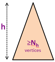
Let N_h be the minimum number of vertices in a height-balanced AVL Tree of height h.

The first few values of N_h are N₀ = 1 (a single root vertex), N₁ = 2 (a root vertex with either one left child or one right child only), N₂ = 4, N₃ = 7, N₄ = 12, N₅ = 20 (see the background picture), and so on (see the next two slides).

We know that for any other AVL Tree of N vertices (not necessarily the minimum-size one), we have N ≥ N_h.

In the background picture, we have N₅ = 20 vertices but we know that we can squeeze 43 more vertices (up to N = 63) before we have a perfect binary tree of height h = 5.

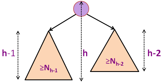
Nh = 1 + Nh-1 + Nh-2 (formula for minimum-size AVL tree of height h)
Nh > 1 + 2*Nh-2 (as Nh-1 > Nh-2)
Nh > 2*Nh-2 (obviously)
Nh > 4*Nh-4 (recursive)
Nh > 8*Nh-6 (another recursive step)
... (we can only do this h/2 times, assuming initial h is even)
Nh > 2h/2*N0 (we reach base case)
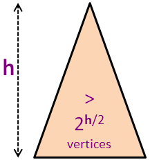
Nh > 2h/2 (as N0 = 1)

N ≥ Nh > 2h/2 (combining the previous two slides)
N > 2h/2
log2(N) > log2(2h/2) (log2 on both sides)
log2(N) > h/2 (formula simplification)
2 * log2(N) > h or h < 2 * log2(N)
h = O(log(N)) (the final conclusion)

Look at the example BST again. See that all vertices are height-balanced, an AVL Tree.

To quickly detect if a vertex v is height balanced or not, we modify the AVL Tree invariant (that has absolute function inside) into: bf(v) = v.left.height - v.right.height.

Now try Insert(37) on the example AVL Tree again. A few vertices along the insertion path: {41,20,29,32} increases their height by +1. Vertices {29,20} will no longer be height-balanced after this insertion (and will be rotated later — discussed in the next few slides), i.e. bf(29) = -2 and bf(20) = -2 too. We need to restore the balance.

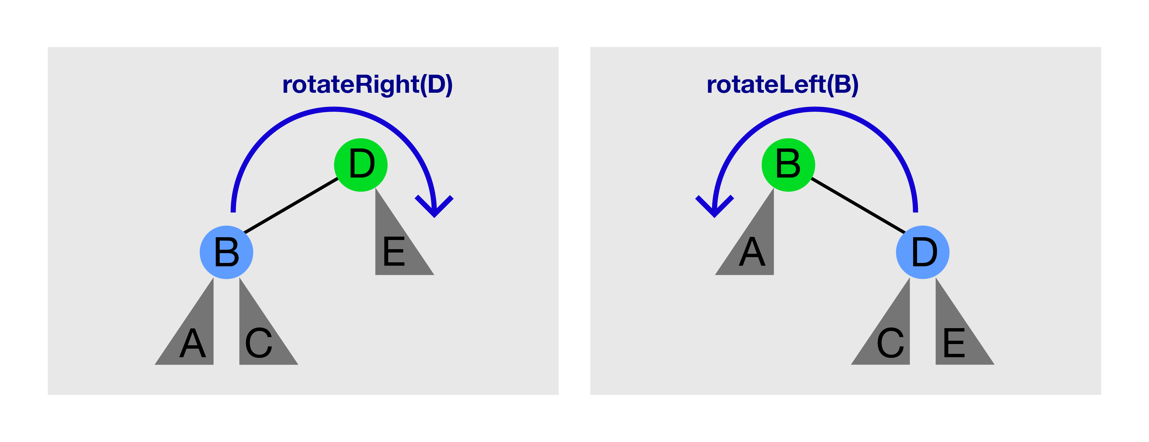
See the picture above. Calling rotateRight(D) on the left picture will produce the right picture. Calling rotateLeft(B) on the right picture will produce the left picture again.

rotateRight(T)/rotateLeft(T) can only be called if T has a left/right child, respectively.

Tree Rotation preserves BST property.
Before rotation, A < B < C < D < E.
After rotation, notice that subtree rooted at C (if it exists) changes parent,
but the order of A < B < C < D < E does not change.

BSTVertex rotateLeft(BSTVertex T) // pre-req: T.right != null
  BSTVertex w = T.right // rotateRight is the mirror copy of this
  w.parent = T.parent // this method is hard to get right for newbie
  T.parent = w
  T.right = w.left
  if (w.left != null) w.left.parent = T
  w.left = T
  // update the height of T and then w here
  return w

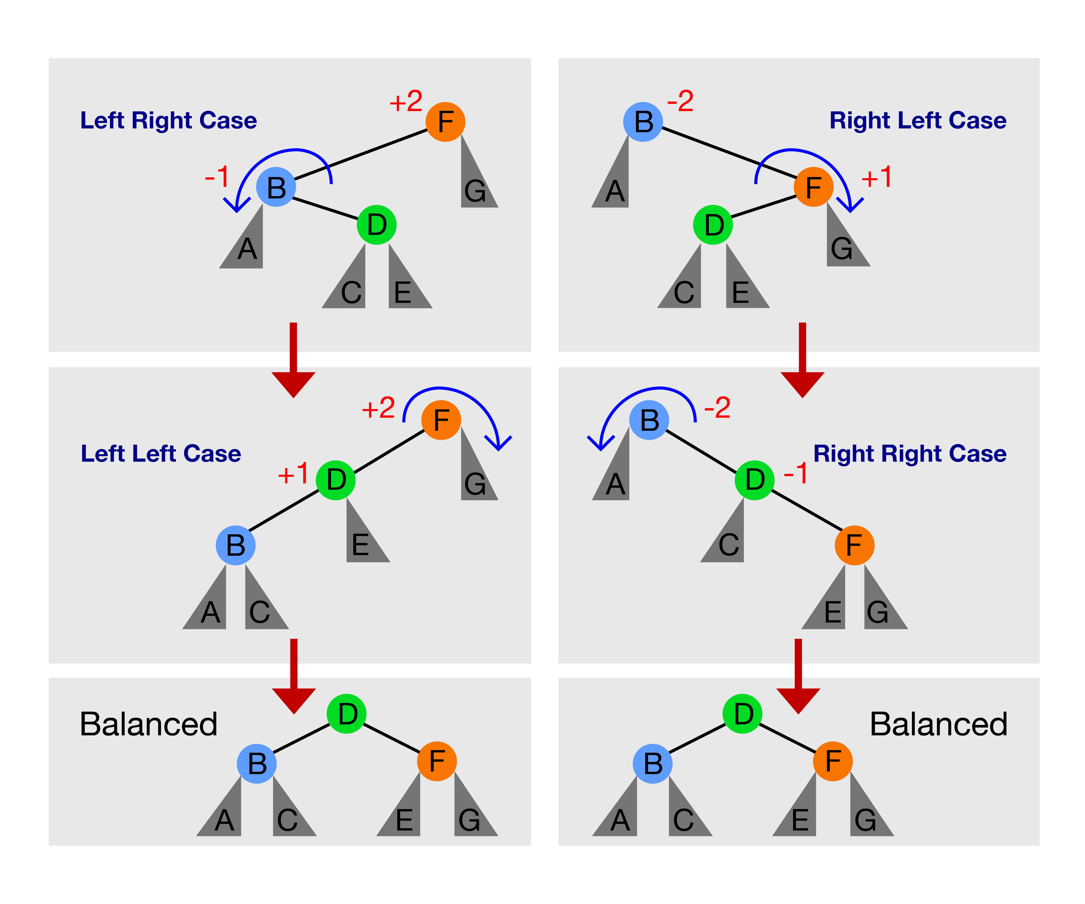
There are only these four cases:

1. Left Left Case: bf(F) = +2 and bf(D) = +1, solution: rotateRight(F)
2. Left Right Case: bf(F) = +2 and bf(B) = -1, solution: rotateLeft(B) first to transform this case into Left Left Case again, then go to step 1
3. Right Right Case: bf(B) = -2 and bf(D) = -1, solution: rotateLeft(B)
4. Right Left Case: bf(B) = -2 and bf(F) = +1, solution: rotateRight(F) first to transform this case into Right Right Case again, then go to step 3

1. Just insert v as in normal BST,
2. Walk up the AVL Tree from the insertion point back to the root and at every step, we update the height and balance factor of the affected vertices:
   1. Stop at the first vertex that is out-of-balance (+2 or -2), if any,
   2. Use one of the four tree rotation cases to rebalance it again, e.g. try Insert(37) on the example above and notice by calling rotateLeft(29) once, we fix the imbalance issue.

Discussion: Is there other tree rotation cases for Insert(v) operation of AVL Tree?

1. Just remove v as in normal BST (one of the three removal cases),
2. Walk up the AVL Tree from the deletion point back to the root and at every step, we update the height and balance factor of the affected vertices:
   1. Now for every vertex that is out-of-balance (+2 or -2), we use one of the four tree rotation cases to rebalance them (can be more than one) again.

The main difference compared to Insert(v) in AVL tree is that we may trigger one of the four possible rebalancing cases several times, but not more than h = O(log N) times :O, try Remove(7) on the example above to see two chain reactions rotateRight(6) and then rotateRight(16)+rotateLeft(8) combo.

We have now see how AVL Tree defines the height-balance invariant, maintain it for all vertices during Insert(v) and Remove(v) update operations, and a proof that AVL Tree has h < 2 * log N.

Therefore, all BST operations (both update and query operations except Inorder Traversal) that we have learned so far, if they have time complexity of O(h), they have time complexity of O(log N) if we use AVL Tree version of BST.

This marks the end of this e-Lecture, but please switch to 'Exploration Mode' and try making various calls to Insert(v) and Remove(v) in AVL Tree mode to strengthen your understanding of this data structure.

PS: If you want to study how these seemingly complex AVL Tree (rotation) operations are implemented in a real program, you can download this AVLDemo.cpp | java (must be used together with this BSTDemo.cpp | java).

We will end this module with a few more interesting things about BST and balanced BST (especially AVL Tree).

For a few more interesting questions about this data structure, please practice on BST/AVL training module (no login is required).

However, for registered users, you should login and click the training icon from the homepage to officially clear this module and such achievement will be recorded in your user account.

We also have a few programming problems that somewhat requires the usage of this balanced BST (like AVL Tree) data structure: Kattis - compoundwords and Kattis - baconeggsandspam.

Try them to consolidate and improve your understanding about this data structure. You are allowed to use C++ STL map/set, Java TreeMap/TreeSet, or OCaml Map/Set if that simplifies your implementation (Note that Python doesn't have built-in bBST implementation).