
排序问题有许多有趣的算法解决方案,体现了许多计算机科学的思想:
When an (integer) array A is sorted, many problems involving A become easy (or easier), please review the applications, the slower/harder unsorted array solutions, and the faster/easier sorted array solutions.
第二个操作是最重要的操作:通过单击“Sort”按钮来执行排序算法。
需要注意的是,你可以通过切换页面顶部的算法缩写来切换当前算法。
为了节省屏幕空间,我们将算法名称缩写为三个字符:
在接下来的幻灯片,我们将讨论三种基于比较的排序算法
你应该已经了解下列知识:
-. 对数和指数, e.g., log2(1024) = 10, 210 = 1024
-. 等差数列, e.g., 1+2+3+4+…+10 = 10*11/2 = 55
-. 等比数列, e.g., 1+2+4+8+..+1024 = 1*(1-211)/(1-2) = 2047
-. 线性/二次/三次函数, e.g., f1(x) = x+2, f2(x) = x2+x-1, f3(x) = x3+2x2-x+7
-. 向上取整 (ceiling), 向下取整 (floor) , 和绝对值 (absolute) 函数, e.g., ceil(3.1) = 4, floor(3.1) = 3, abs(-7) = 7
我们可以通过使用墙钟时间或在我们的程序中插入时间测量代码来测量程序的实际运行时间,例如,参见 SpeedTest.cpp | py | java 中显示的代码。
然而,实际运行时间在比较两种算法时并没有意义,因为它们可能是用不同的语言编写的,使用不同的数据集,或在不同的计算机上运行。
我们不是测量实际的时间,而是计算操作的数量(算术,赋值,比较等)。这是一种评估其效率的方法,因为算法的执行时间与它所需的操作数量有关。
请参阅在 SpeedTest.cpp | py | java 中显示的代码和评论(特别是如何获得变量计数器的最终值)。
知道算法需要的操作数量(精确),我们可以这样说:算法 X 需要 2n2 + 100n 次操作来解决大小为 n 的问题。
如果已知一次操作所需的时间t,那么我们可以说算法X需要(2n2 + 100n)t时间单位来解决大小为n的问题。
然而,时间t取决于前面提到的因素,例如,不同的语言、编译器和计算机,操作本身的复杂性(加法/减法比乘法/除法更容易/更快地计算),等等。
因此,我们可以说,算法X解决大小为n的问题所需的时间与2n2 + 100n成比例,而不是将分析与实际时间t绑定在一起。
渐近分析是一种专注于分析大输入大小n问题的算法分析,只考虑公式的主导项,并忽略主导项的系数。
我们选择主导项,因为随着输入的增大,低阶项对总体成本的贡献较小,例如,对于f(n) = 2n2 + 100n,我们有:
f(1000) = 2*10002 + 100*1000 = 2.1M,相比之下
f(100000) = 2*1000002 + 100*100000 = 20010M。
(注意,低阶项100n的贡献较小)。
写作算法 A 有时间复杂度 O(f(n)),其中 f(n) 是算法 A 的增长率函数。
method bubbleSort(array A, integer N) // 标准版本
  for each R from N-1 down to 1 // 重复 N-1 次迭代
    for each index i in [0..R-1] // '未排序区域',O(N)
      if A[i] > A[i+1] // 这两个不是非递减顺序
        swap(a[i], a[i+1]) // 在 O(1) 中交换它们
比较和交换需要的时间由一个常数限制,我们称之为 c。然后,在(标准)冒泡排序中有两个嵌套循环。外循环正好运行 N-1 次迭代。但是内循环的运行时间越来越短:
因此,总的迭代次数 = (N−1)+(N−2)+...+1 = N*(N−1)/2 (推导).
总时间 = c*N*(N−1)/2 = O(N^2).
请参阅在 SortingDemo.cpp | py | java 中显示的代码。
冒泡排序实际上效率低下,其O(N^2)时间复杂度。想象一下,我们有N = 105个数字。即使我们的计算机超级快,能在1秒内计算108次操作,冒泡排序也需要大约100秒才能完成。
然而,它可以提前终止,例如,在上面显示的小型升序排序示例 [3, 6, 11, 25, 39]中,可以在O(N)时间内终止。
改进的想法很简单:如果我们在内循环中没有交换,那就意味着数组已经排序,我们可以在那个点停止冒泡排序。
讨论:尽管这使冒泡排序在一般情况下运行得更快,但这个改进的想法并没有改变冒泡排序的O(N^2)时间复杂度...为什么呢?
method selectionSort(array A[], integer N)
  for each L in [0..N-2] // O(N)
    let X be the index of the minimum element in A[L..N-1] // O(N)
    swap(A[X], A[L]) // O(1),X 可能等于 L (没有实际交换)
总计: O(N2) — 准确地说,它类似于冒泡排序分析。
请参阅在SortingDemo.cpp | py | java中显示的代码。
Quiz: How many (real) swaps are required to sort [29, 10, 14, 37, 13] by Selection Sort?
插入排序类似于大多数人整理扑克牌的方式。
让我们尝试在小示例数组 [40, 13, 20, 8] 上使用 。
method insertionSort(array A[], integer N)
  for i in [1..N-1] // O(N)
    let X be A[i] // X is the next item to be inserted into A[0..i-1]
    for j from i-1 down to 0 // this loop can be fast or slow
      if A[j] > X
        A[j+1] = A[j] // make a place for X
      else
        break
    A[j+1] = X // insert X at index j+1
See the code shown in SortingDemo.cpp | py | java.
Quiz: What is the complexity of Insertion Sort on any input array?
我们将在接下来的几张幻灯片中讨论两种基于比较的排序算法:
method merge(array A, integer low, integer mid, integer high)
  // 子数组1 = a[low..mid], 子数组2 = a[mid+1..high], 都已排序
  int N = high-low+1
  create array B of size N // 讨论:为什么我们需要一个临时数组b?
  int left = low, right = mid+1, bIdx = 0
  while (left <= mid && right <= high) // 合并过程
    if (A[left] <= A[right])
      B[bIdx++] = A[left++]
    else
      B[bIdx++] = A[right++]
  while (left <= mid)
    B[bIdx++] = A[left++] // 剩余部分,如果有的话
  while (right <= high)
    B[bIdx++] = A[right++] // 剩余部分,如果有的话
  for (int k = 0; k < N; ++k)
    A[low+k] = B[k]; // 复制回去
尝试在示例数组 [1, 5, 19, 20, 2, 11, 15, 17] 上使用 ,该数组的前半部分已经排序 [1, 5, 19, 20],其后半部分也已经排序 [2, 11, 15, 17]。请集中注意力在归并排序算法的最后一次合并。
归并并排序是分而治之的排序算法。
划分步骤很简单:将当前数组分成两半(如果 N 是偶数,则将其完全平等,或者如果 N 是奇数,则一边多一项),然后递归地对这两半进行排序。
解决步骤是主要的工作:使用前面讨论的归并子程序合并两个(排序的)半部分以形成一个有序数组。
method mergeSort(array A, integer low, integer high)
  // 要排序的数组是 A[low..high]
  if (low < high) // 基本情况:low >= high (0 或 1 个项目)
    int mid = (low+high) / 2
    mergeSort(a, low  , mid ) // 分成两半
    mergeSort(a, mid+1, high) // 然后递归排序它们
    merge(a, low, mid, high) // 征服:合并子程序
请参阅在SortingDemo.cpp | py | java中显示的代码。
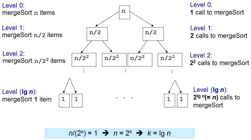
无论输入的原始顺序如何,归并排序中最重要的部分是其O(N log N)性能保证。 就这样,没有任何针对性的测试用例可以使归并排序对于N个元素数组运行比O(N log N)更长的时间。
因此,归并排序非常适合大数组的排序,因为O(N log N)比前面讨论的O(N2)排序算法增长得慢得多。
然而,归并排序有几个不太好的部分。 首先,从零开始实现并不容易(虽然我们不必这样做)。 其次,它在归并操作期间需要额外的O(N)内存,因此会占用额外内存并且不是就地的 (in-place)。顺便说一句,如果你有兴趣看看为解决这些(经典)归并排序不那么好的部分做了什么,你可以阅读这个。
归并排序也是一个稳定 (stable) 的排序算法。 讨论:为什么?
快速排序是另一个分而治之的排序算法(另一个在这个可视化页面中讨论的是归并排序)。
在继续随机化和可用版本的快速排序之前,我们将看到,这种确定性的,非随机化的快速排序的版本可能在针对性输入中具有很差的 O(N2) 时间复杂度。
划分步骤:选择一个项目p(称为枢轴)
然后将A[i..j]的项目划分为三部分:A[i..m-1],A[m]和A[m+1..j]。
A[i..m-1](可能为空)包含小于(或等于)p的项目。
A[m] = p,即,索引m是数组a排序顺序中p的正确位置。
A[m+1..j](可能为空)包含大于(或等于)p的项目。
然后,递归排序这两部分。
征服步骤:别惊讶...我们什么都不做 :O!
如果你将这个与合并排序进行比较,你会发现快速排序的D&C步骤与合并排序完全相反。
我们将通过首先讨论其最重要的子程序:O(N) partition(经典版本)来剖析这个快速排序算法。
要划分A[i..j],我们首先选择A[i]作为枢轴p。
剩余的项目(即,a[i+1..j])被划分为3个区域:
讨论:为什么我们选择p = A[i]?还有其他选择吗?
更难的讨论:如果A[k] == p,我们应该将它放在区域S1还是S2?
最初,S1 和 S2 区域都是空的,即所有除指定的轴心 p 之外的项目都在未知区域。
然后,对于未知区域中的每个项目 A[k],我们将 A[k] 与 p 进行比较,并决定以下三种情况之一:
这三种情况将在接下来的两张幻灯片中详细说明。
最后,我们交换 A[i] 和 A[m],将轴心 p 正好放在 S1 和 S2 的中间。
![Case when a[k] ≥ p, increment k, extend S2 by 1 item](https://visualgo.net/img/partition1.png)
![Case when a[k] < p, increment m, swap a[k] with a[m], increment k, extend S1 by 1 item](https://visualgo.net/img/partition2.png)
int partition(array A, integer i, integer j)
  int p = a[i] // p 是枢轴
  int m = i // S1 和 S2 最初为空
  for (int k = i+1; k <= j; ++k) // 探索未知区域
    if ((A[k] < p) || ((A[k] == p) && (rand()%2 == 0)))  { // 情况 2+3
      ++m
      swap(A[k], A[m]) // 交换这两个索引
    // 注意我们在情况 1: A[k] > p 时不做任何事情
  swap(A[i], A[m]) // 最后一步,交换枢轴和 a[m]
  return m // 返回枢轴的索引
method quickSort(array A, integer low, integer high)
  if (low < high)
    int m = partition(a, low, high) // O(N)
    // A[low..high] ~> A[low..m–1], pivot, A[m+1..high]
    quickSort(A, low, m-1); // 递归排序左子数组
    // A[m] = pivot 在分区后已经排序
    quickSort(A, m+1, high); // 然后排序右子数组
请参阅在SortingDemo.cpp | py | java中显示的代码。
尝试在示例数组 [27, 38, 12, 39, 29, 16] 上使用 。我们将详细说明第一步分区操作如下:
我们设定 p = A[0] = 27。
我们设定 A[1] = 38 作为 S2 的一部分,所以 S1 = {} 和 S2 = {38}。
我们交换 A[1] = 38 和 A[2] = 12,所以 S1 = {12} 和 S2 = {38}。
我们设定 A[3] = 39 和后来的 A[4] = 29 作为 S2 的一部分,所以 S1 = {12} 和 S2 = {38,39,29}。
我们交换 A[2] = 38 和 A[5] = 16,所以 S1 = {12,16} 和 S2 = {39,29,38}。
我们交换 p = A[0] = 27 和 A[2] = 16,所以 S1 = {16,12},p = {27},和 S2 = {39,29,38}。
之后,A[2] = 27 保证已经排序,现在快速排序递归地首先排序左边的 A[0..1],然后递归地排序右边的 A[3..5]。
首先,我们分析一次partition调用的成本。
在partition(A, i, j)中,只有一个for循环,它迭代了(j-i)次。由于j可以大到N-1,i可以小到0,所以partition的时间复杂度是O(N)。
类似于归并排序分析,快速排序的时间复杂度则取决于partition(A, i, j)被调用的次数。
当数组A已经按升序排列,例如,A = [5, 18, 23, 39, 44, 50], 将设置p = A[0] = 5,并返回m = 0,从而使S1区域空,S2区域:除了枢轴(N-1 项)以外的所有其他内容。
在这种最坏情况的输入场景下,会发生以下情况:
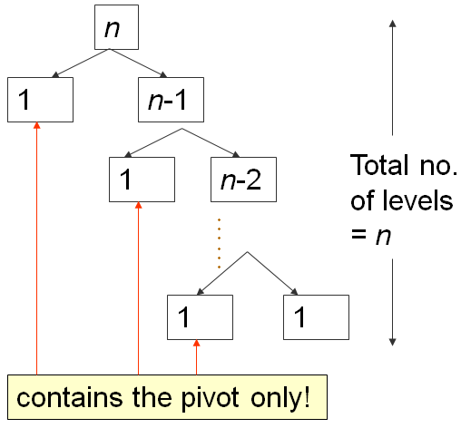
第一次分区需要 O(N) 的时间,将 A 分为 0, 1, N-1 个项目,然后向右递归。
第二次分区需要 O(N-1) 的时间,将 A 分为 0, 1, N-2 个项目,然后再次向右递归。
...
直到最后,第 N 次分区将 A 分为 0, 1, 1 个项目,快速排序递归停止。
这是经典的 N+(N-1)+(N-2)+...+1 模式,它是 O(N2),与这个冒泡排序分析幻灯片中的分析类似...
当分区总是将数组分成两个相等的一半时,就会发生快速排序的最佳情况,如归并排序。
当发生这种情况时,递归的深度只有 O(log N)。
由于每个级别进行 O(N) 比较,时间复杂度为 O(N log N)。
在这个手工制作的示例输入数组 [4, 1, 3, 2, 6, 5, 7] 上尝试。这在实践中很少见,因此我们需要设计一个更好的方法:随机快速排序。
与快速排序相同,除了在执行分区算法之前,它随机选择A[i..j]之间的枢轴,而不是总是确定性地选择A[i](或[i..j]之间的任何其他固定索引)。
小练习:将上述想法应用到这个幻灯片中显示的实现!
在这个大而有些随机的示例数组a = [3,44,38,5,47,15,36,26,27,2,46,4,19,50,48]上运行 感觉很快。
要正确解释为什么这个随机版本的快速排序在任何包含N个元素的输入数组上的预期时间复杂度为O(N log N),大约需要1小时的讲座。
在这个电子讲座中,我们将假设这是正确的。
如果你需要非正式的解释:只需想象在随机化版本的快速排序中,我们随机选择枢轴,我们不总是得到极其糟糕的分割,即0(空),1(枢轴),和N-1个其他项目。这种幸运(半枢轴半),有点幸运,有点不幸,和极其不幸(空,枢轴,其余)的组合产生了平均时间复杂度为O(N log N)。
讨论:对于Partition的实现,如果A[k] == p,我们总是确定性地将A[k]放在一侧(S1或S2)会发生什么?
在接下来的幻灯片,我们将讨论两种不基于比较的排序算法:
这些排序算法可以不比较数组的项,从而比时间复杂度为 Ω(N log N)的基于比较的排序算法的下限更快。
众所周知(尽管在这个可视化中并未证明,因为这需要大约半小时的决策树模型讲座才能做到),所有基于比较的排序算法的时间复杂度下界都是Ω(N log N)。
因此,任何具有最坏情况复杂度为O(N log N)的基于比较的排序算法,如Merge Sort,都被认为是最优算法,即我们不能做得比这更好。
然而,如果输入数组存在某些假设,我们可以实现更快的排序算法 — 即O(N) — 从而避免比较项目以确定排序顺序。
假设:如果要排序的项目是具有大范围但少位数的整数,我们可以将计数排序的思想与基数排序相结合,以实现线性时间复杂度。
在基数排序中,我们将要排序的每个项目视为一个由w位数字组成的字符串(如果需要,我们会在位数少于w位的整数前面填充零)。
从最低有效位(最右边)到最高有效位(最左边),我们遍历N个项目,并根据当前位将它们放入10个队列中(每个数字[0..9]一个队列),这类似于一个修改过的计数排序,因为它保持了稳定性(请记住,之前在此幻灯片中展示的计数排序版本不是稳定排序)。然后我们再次将这些组重新连接起来进行后续迭代。
尝试在上面的随机4位数数组上点击 以获得更清晰的解释。
请注意,我们只执行了O(w × (N+k))次迭代。在这个例子中,w = 4,k = 10。
现在,我们已经讨论过基数排序,那么我们应该在每一个排序情况下使用它吗?
例如,理论上来说,对许多(N非常大)32位有符号整数进行排序应该更快,因为w ≤ 10位数,k = 10,如果我们将这些32位有符号整数解释为十进制。O(10 × (N+10)) = O(N)。
讨论:如本可视化所示,使用基数10实际上并不是排序N个32位有符号整数的最佳方式。那么更好的设置应该是什么呢?
如果一个排序算法在排序过程中只需要常量级别(即,O(1))的额外空间,那么我们就说这是一个原地排序算法。也就是说,少量的、常数个数的额外变量是可以的,但我们不允许有依赖于输入大小N的变量长度。
归并排序(经典版本),由于其merge子程序需要额外的临时数组,大小为N,所以它不是原地排序。
讨论:冒泡排序、选择排序、插入排序、快速排序(是否随机)、计数排序和基数排序,哪些是原地排序?
如果排序算法在排序执行后保留了具有相同键值的元素的相对顺序,那么这种排序算法被称为稳定(stable)。
稳定排序的示例应用:假设我们有按字母顺序排序的学生名字。现在,如果这个列表再次按照教学小组编号排序(回想一下,一个教学小组通常有很多学生),一个稳定的排序算法会确保同一个教学小组的所有学生仍然按照他们的名字的字母顺序出现。基数排序需要通过多轮按位排序,并需要一个稳定的排序子程序才能正确工作。
讨论:在这个电子讲座中讨论的排序算法中,哪些是稳定的?
尝试对数组 A = {3, 4a, 2, 4b, 1} 进行排序,即有两个4的副本(先是4a,然后是4b)。
Quiz: Which of these algorithms run in O(N log N) on any input array of size N?
Quiz: Which of these algorithms has worst case time complexity of Θ(N^2) for sorting N integers?
Bubble Sort我们已经到了电子讲座 - 排序的末尾。
但是,VisuAlgo 中还有另外两种嵌入在其他数据结构中的排序算法:堆排序和平衡BST排序。 我们将在这两种数据结构的电子讲座里面讨论它们。
实际上,许多这些基本排序算法的C ++源代码已经分散在这些电子讲座幻灯片中。对于其他编程语言,您可以将给定的C ++源代码翻译为其他编程语言。
通常,排序只是问题解决过程中的一小部分,而现在大多数编程语言都有自己的排序函数,所以非必要情况,我们不需要复现其代码。
在C++中,您可以使用STL算法中的std::sort,std::stable_sort 或 std::partial_sort。
在Java中,您可以使用Collections.sort。
在Python中,您可以使用sort。
在OCaml中,您可以使用List.sort compare list_name。
如果比较函数是针对特定问题的,我们可能需要为这些内置的排序例程提供额外的比较函数。
Now it is time for you to see if you have understand the basics of various sorting algorithms discussed so far.
Test your understanding here.
现在您已经到了电子讲座的最后部分,您认为排序问题与调用内置的排序程序一样简单吗?
尝试这些在线评判问题以了解更多信息:
Kattis - mjehuric
Kattis - sortofsorting,或者
Kattis - sidewayssorting
这不是排序算法的结束。 当您在 VisuAlgo 中探索其他主题时,您会意识到排序是许多其他高难度问题的高级算法的预处理步骤,例如, 作为克鲁斯卡尔算法(Kruskal's algorithm)的预处理步骤,创造性地用于后缀数组 (Suffix Array) 数据结构等。
start of 3230 material