二叉堆是实现高效优先队列(PQ)抽象数据类型(ADT)的一种可能的数据结构。在PQ中,每个元素都有一个“优先级”,优先级较高的元素在优先级较低的元素之前被服务(平局可以简单地随意解决,或者按照普通队列的先进先出(FIFO)规则解决)。尝试点击 ,查看上面随机二叉堆提取最大值的示例动画。
为了集中讨论范围,这个可视化展示了一个允许重复的整数二叉最大堆。查看这个,了解如何轻松转换为二叉最小堆。通常,任何可以比较的其他对象都可以存储在二叉最大堆中,例如,浮点数的二叉最大堆等。
完全二叉树:二叉树中的每一层,除了可能的最后/最低层,都被完全填满,且最后一层的所有顶点尽可能地靠左。
二叉最大堆属性:每个顶点的父顶点(除了根)包含的值大于(或等于 —— 我们现在允许重复)该顶点的值。这比以下的替代定义更容易验证:一个顶点的值(除了叶子/叶子)必须大于(或等于)其一个(或两个)子节点的值。
优先队列 (PQ) 抽象数据类型 (ADT) 与普通队列 ADT 类似,但有以下两个主要操作:
讨论:一些 PQ ADT 在 PQ 中最高优先级(键)并列的情况下,会恢复到普通队列的先进先出 (FIFO) 行为。保证在最高优先级(键)相等的情况下的稳定性是否使 PQ ADT 更难实现?
想象一下:你是一名在机场控制塔T工作的空中交通管制员 (ATC)。你已经安排飞机X/Y分别在接下来的3/6分钟内降落。两架飞机的燃料都足够飞行至少接下来的15分钟,而且都离你的机场只有2分钟的路程。你观察到你的机场跑道目前是清晰的。

如果你不知道,飞机可以被指示在机场附近保持飞行模式,直到指定的降落时间。
你必须参加现场讲座才能弄清楚接下来会发生什么...
将向你提供两个选项,你需要做出决定:
如果这两个选项都不合理,那就什么都不做。
除了你刚才看到的关于ATC(仅在现场讲座中)的内容外,优先队列 ADT在现实生活中还有几种潜在的用途。
讨论:你能提出几个其他需要优先队列的现实生活情况吗?
We are able to implement this PQ ADT using (circular) Array or Linked List but we will have slow (i.e., in O(N)) Enqueue or Dequeue operation.
Discussion: Why?
Now, let's view the visualisation of a (random) Binary (Max) Heap above. You should see a complete binary tree and all vertices except the root satisfy the Max Heap property (A[parent(i)] ≥ A[i]). Duplicate integer keys may appear (note that the stability of equal keys is not guaranteed).
You can between the visually more intuitive complete binary tree form or the compact array based implementation of a Binary (Max) Heap.
Quiz: Based on this Binary (Max) Heap property, where will the largest integer be located?
完全二叉树可以作为紧凑数组A有效地存储,因为完全二叉树的顶点/紧凑数组的元素之间没有间隙。为了简化下面的导航操作,我们使用基于1的数组。VisuAlgo在每个顶点下方以红色标签显示每个顶点的索引。按照从1到N的排序顺序阅读这些索引,然后你会看到从上到下,从左到右的完全二叉树的顶点。为了帮助你理解这一点,几次。
这样,我们可以使用简单的索引操作(借助位移操作的帮助)实现基本的二叉树遍历操作:
专业提示:尝试在两个浏览器窗口上打开两个VisuAlgo的副本。尝试在两种不同的模式下可视化同一个二叉最大堆,并进行比较。
在这个可视化中,你可以执行几个二叉(最大)堆操作:
还有一些其他可能的二叉(最大)堆操作,但是我们目前在某个NUS模块中出于教学原因并未详细说明。
Insert(v): 当我们在往最大二叉堆插入元素 v 的时候 我们只能插入到最后一个元素 N + 1 来维持一个紧凑的数组 = 完整二叉树特性。然而 最大堆的特性仍然可能没被满足。这时我们从插入点往上去修复最大堆特性(如果需要的话)直到整个堆符合最大堆特性。现在点 几次来插入几个随机的 v 进去现在显示的最大二叉堆。
这个向上走并且修复最大堆特性的操作没有公认的名字。我们叫它 ShiftUp (上移)但是还有人叫它 BubbleUp 或者 IncreaseKey 操作.
Insert(v) 的时间复杂度是 O(log N)。
讨论:你理解这个推论吗?
ExtractMax(): 提取并删除最大二叉堆中的最大元素(根)的操作需要一个在堆中的元素来替换根,不然最大堆(一个完整的二叉树,在中文中的'林‘)会变成两个断开的子树(中文中两个'木’)。这同样也是这个元素必须是最后一个元素N的原因:维持紧凑数组 = 完整二叉树性质。
因为我们要把最大二叉堆中的一个叶顶点晋升成根顶点,它很可能是会违背最大堆特性。ExtractMax() 这时从根往下比较当前值和它的两个子元素的值(如果必要的话)来修复最大二叉堆特性。现在在当前显示的最大二叉堆中试试
这个向下走并修复最大堆特性的操作没有公认的名字。我们叫它 ShiftDown (下移)但是还有人叫它 BubbleDown 或者 Heapify 操作。.
ExtractMax() 的时间复杂度是 O(log N)。
讨论:你理解这个推论吗?
到目前为止,我们有一个数据结构,可以有效地实现优先队列 (PQ) ADT的两个主要操作:
然而,我们可以用二叉堆做更多的操作。
Create(A): 用含有 N 个逗号分隔的数组 A 从一个空的最大二叉堆开始创建一个合法的最大二叉堆
有两种方法完成创建操作一个简单但是慢 -> O(N log N) 另一个用更复杂的技术但是快 -> O(N).
教你一招:在两个浏览器里面同时打开 VisuAlgo。用最差情况 '已排序例子' 去执行不同版本的 Create(A),你会看到可怕的差距。
Create(A) - O(N log N):简单地插入(即,通过调用 Insert(v) 操作)输入数组中的所有 N 个整数到一个最初为空的二叉最大堆中。
分析:这个操作显然是 O(N log N),因为我们调用 O(log N) Insert(v) 操作 N 次。让我们来看看 '排序示例',这是这个操作的一个难点(现在试试 ,我们展示了一个案例,其中 A = [1,2,3,4,5,6,7] -- 请耐心等待,因为这个示例需要一些时间来完成)。如果我们按递增顺序将值插入到一个最初为空的二叉最大堆中,那么每次插入都会触发一条从插入点(一个新的叶子)向上到根的路径。
Create(A) - O(N): This faster version of Create(A) operation was invented by Robert W. Floyd in 1964. It takes advantage of the fact that a compact array = complete binary tree and all leaves (i.e., half of the vertices — see the next slide) are Binary Max Heap by default. This operation then fixes Binary Max Heap property (if necessary) only from the last internal vertex back to the root.
Analysis: A loose analysis gives another O(N/2 log N) = O(N log N) complexity but it is actually just O(2*N) = O(N) — details here. Now try the on the same input array A = [1,2,3,4,5,6,7] and see that on the same hard case as with the previous slide (but not the one that generates maximum number of swaps — try 'Diagonal Entry' test case), this operation is far superior than the O(N log N) version.
简单证明为什么在最大堆中(里面N个元素)一半的元素都是叶元素(为了概括性,我们假设N是偶数):
假设最后一个叶元素的序号是 N, 那么它的父元素的序号是 i = N/2 (回忆 这节课). 它的左子元素的序号是 i+1, 如果存在的话 (它其实并不存在), 将会是 2*(i+1) = 2*(N/2+1) = N+2, 这个结果超过了 N (最后一个叶元素) 所以 i+1 一定是一个没有子元素的叶元素。因为二叉堆的序号是连续的,所以序号s [i+1 = N/2+1, i+2 = N/2+2, ..., N], 或者说一半的顶点,都是叶元素。
堆排序函数HeapSort(): John William Joseph Williams 在1964年发明了堆排序算法和这个二叉堆数据结构. 堆排序的操作 (假定最大二叉堆已经在O(n)的时间复杂度内建立)非常简单。只需要调用提取堆顶函数ExtractMax() n次即可,每次的时间复杂度为O(log N). 现在你可以试一下屏幕上的这个最大二叉堆
Quiz: In worst case scenario, HeapSort() is asymptotically faster than...
Insertion Sort尽管 HeapSort() 在最好/平均/最坏 情况下的时间复杂度都是 θ(N log N) ,它真的是最好的用比较元素的方法来实现的排序算法吗?
讨论点:HeapSort()的缓存性能如何?
当你全部学会了的时候,我们邀请你学习更高级的算法,它们用优先队做底层数据结构(之一),例如 Prim's MST algorithm, Dijkstra's SSSP algorithm, A* 搜索算法(还不在 VisuAlgo里), 一些贪婪算法,等等.
Earlier, we have seen that we can create Binary Max Heap from a random array of size N elements in O(N) instead of O(N log N). Now, we will properly analyze this tighter bound.
First, we need to recall that the height of a full binary tree of size N is log2 N.
Second, we need to realise that the cost to run shiftDown(i) operation is not the gross upper bound O(log N), but O(h) where h is the height of the subtree rooted at i.
Third, there are ceil(N/2h+1) vertices at height h in a full binary tree.
On the example full binary tree above with N = 7 and h = 2, there are:
ceil(7/20+1) = 4 vertices: {44,35,26,17} at height h = 0,
ceil(7/21+1) = 2 vertices: {62,53} at height h = 1, and
ceil(7/22+1) = 1 vertex: {71} at height h = 2.
Cost of Create(A), the O(N) version is thus:
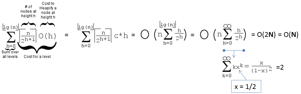
PS: If the formula is too complicated, a modern student can also use WolframAlpha instead.
The faster O(N) Create Max Heap from a random array of N elements is important for getting a faster solution if we only need top K elements out of N items, i.e., PartialSort().
After O(N) Create Max Heap, we can then call the O(log N) ExtractMax() operation K times to get the top K largest elements in the Binary (Max) Heap. Now try on the currently displayed Binary (Max) Heap.
Analysis: PartialSort() clearly runs in O(N + K log N) — an output-sensitive algorithm where the time complexity depends on the output size K. This is faster than the lower-bound of O(N log N) if we fully sort the entire N elements when K < N.
If there are duplicate keys, the standard implementation of Binary Heap as shown in this visualization does not guarantee stability. For example, if we insert three copies of {7, 7, 7}, e.g., {7a, 7b, and 7c} (suffix a, b, c are there only for clarity), in that order, into an initially empty Binary (Max) Heap. Then, upon first extraction, the root (7a) will be extracted first and the last existing leaf (7c) will replaces 7a. As 7c and 7b (without the suffixes) are equal (7 and 7), there is no swap happening and thus the second extract max will take out 7c instead of 7b first — not stable.
If we really need to guarantee stability of equal elements, we probably need to attach different suffixes as shown earlier to make those identical elements to be unique again.
如果你正在寻找二叉(最大)堆的实现来实际模拟优先队列,那么有个好消息。
C++ 和 Java 已经有内置的优先队列实现,很可能使用了这种数据结构。它们是 C++ STL priority_queue(默认是最大优先队列)和 Java PriorityQueue(默认是最小优先队列)。然而,内置的实现可能不适合有效地执行一些 PQ 扩展操作(在某个 NUS 课程中出于教学原因省略了详细信息)。
Python 的 heapq 存在,但其性能相当慢。OCaml 没有内置的优先队列,但我们可以使用将在 VisuAlgo 的其他模块中提到的其他东西(省略详细信息的原因与上述相同)。
附言:堆排序可能用于 C++ STL 算法 partial_sort。
然而,这是我们的 BinaryHeapDemo.cpp | py | java 的实现。
我们还有一些编程问题可以用到二叉堆数据结构UVa 01203 - Argus 和 Kattis - numbertree.
试着解决它们来提高你对这个数据结构的理解。你可以用C++ STL priority_queue, Python heapq或者JAVA PriorityQueue 如果它们可以简化你的解法