Sebuah Pohon Biner Terurut (PBT atau biasa disebut Binary Search Tree, BST dalam Bahasa Inggris) merupakan sebuah pohon biner tipe spesial dengan setiap simpul hanya memiliki tidak lebih dari 2 anak. Struktur data ini memenuhi properti BST, yakni semua simpul-simpul di sub-pohon kiri dari sebuah simpul harus memiliki nilai lebih kecil dibandingkan daripada simpul itu dan semua simpul-simpul di sub-pohon kanan dari sebuah simpul harus memiliki nilai lebih besar daripada simpul itu. Visualisasi ini mengimplementasikan properti 'multiset': walaupun semua kunci mempunyai nilai-nilai berbeda, informasi tentang nilai duplikat disimpan dalam atribut frekuensi (hanya ditunjukkan untuk kunci yang muncul lebih dari sekali). Cobalah mengklik untuk animasi contoh pencarian sebuah nilai acak antara 1 dan 99 inklusif pada BST acak diatas.
Untuk beralih antara BST biasa dan Pohon AVL (dengan perilaku yang berbeda selama Pemasukkan dan Penghapusan dari sebuah bilangan bulat), pilihlah header masing-masing.
Kita juga memiliki shortcut URL untuk dengan cepat mengakses mode Pohon AVL, yaitu https://visualgo.net/en/avl (anda dapat mengganti 'en' ke dua karakter bahasa pilihan anda - jika tersedia).
BST (dan terutama BST yang seimbang seperti Pohon AVL) adalah struktur data efisien untuk mengimplementasikan tipe tertentu dari Struktur Data Abstrak (Abstract Data Type, ADT) Tabel (atau Map).
Sebuah ADT Tabel harus mendukung setidaknya tiga operasi-operasi berikut seefisien mungkin:
Untuk pembahasan yang mirip, anda dapat mengacu pada Kuliah Maya Tabel Hash.
Kami merujuk kepada ADT Tabel yang kunci-kuncinya perlu diurutkan, dibandingkan dengan ADT Tabel yang kunci-kuncinya tidak perlu terurut.
Kebutuhan spesial dari ADT Tabel ini akan diperjelas di beberapa slide-slide seterusnya.
Jika kita menggunakan larik/vector tidak-terurut untuk mengimplementasikan ADT Tabel, hal ini bisa tidak efisien:
Jika kita menggunakan larik/vector terurut untuk mengimplementasikan ADT Tabel, kita dapat memperbaiki performa Cari(v) tetapi melemahkan performa Masukkan(v):
Tunjuan dari Kuliah Maya ini adalah untuk memperkenalkan struktur data BST dan lalu BST yang seimbang (Pohon AVL) sehingga kita dapat mengimplementasikan operasi-operasi dasar dari ADT Tabel: Cari(v), Masukkan(v), Hapus(v), dan beberapa operasi-operasi ADT Tabel lainnya — lihat slide berikutnya — dalam waktu O(log N) — yang adalah jauh lebih kecil dari N.
Catatan: Beberapa dari pembaca yang lebih berpengalaman mungkin menyadari bahwa ∃ struktur data lain yang bisa mengimplementasikan kitiga operasi-operasi dasar ADT Tabel dengan lebih cepat, tapi lanjutkan baca terlebih dulu...
Tunjuan dari Kuliah Maya ini adalah untuk memperkenalkan struktur data BST dan lalu BST yang seimbang (Pohon AVL) sehingga kita dapat mengimplementasikan operasi-operasi dasar dari ADT Tabel: Cari(v), Masukkan(v), Hapus(v), dan beberapa operasi-operasi ADT Tabel lainnya (lihat slide berikutnya) — dalam waktu O(log N). Kompleksitas waktu ini jauh lebih kecil dari N. Silakan coba slider interaktif di bawah ini untuk merasakan perbedaan yang signifikan.
log N = , N = .
Catatan: Beberapa dari pembaca yang lebih berpengalaman mungkin menyadari bahwa terdapat struktur data lain yang bisa mengimplementasikan ketiga operasi-operasi dasar ADT Tabel dengan lebih cepat, tapi lanjutkan baca terlebih dulu...
Diatas tiga operasi dasar, masih ada beberapa operasi-operasi ADT Tabel yang memungkinkan:
Struktur data yang lebih sederhana yang dapat digunakan untuk mengimplementasikan ADT Tabel adalah Linked List.
Quiz: Can we perform all basic three Table ADT operations: Search(v)/Insert(v)/Remove(v) efficiently (read: faster than O(N)) using Linked List?
Diskusi: Kenapa?
Struktur data lainnya yang dapat digunakan untuk mengimplementasikan ADT Tabel adalah Tabel Hash. Struktur data tersebut memiliki performa Cari(v), Masukkan(v), dan Hapus(v) yang sangat cepat (semua dalam ekspektasi kompleksitas waktu O(1)).
Quiz: So what is the point of learning this BST module if Hash Table can do the crucial Table ADT operations in unlikely-to-be-beaten expected O(1) time?
Diskusikan jawaban diatas! Petunjuk: Kembali ke 4 slide sebelumnya.
Kita akan sekarang memperkenalkan struktur data BST. Lihat visualisasi dari BST contoh di atas!
Each vertex has several key attributes: pointer to the left child, pointer to the right child, pointer to the parent vertex, key/value/data, and special for this visualization that implements 'multiset': frequency of each key (there are potential other attributes). Not all attributes will be used for all vertices, e.g., the leaf vertex will have both their left and right child attributes = NULL. Some other implementation separates key (for ordering of vertices in the BST) with the actual satellite data associated with the keys.
The left/right child of a vertex (except leaf) is drawn on the left/right and below of that vertex, respectively. The parent of a vertex (except root) is drawn above that vertex. The (integer) key of each vertex is drawn inside the circle that represent that vertex and if there are duplicated insertion of the same (integer) key, there will be an additional hyphen '-' and the actual frequency (≥ 2) of that key. In the example above, (key) 15 has 6 as its left child and 23 as its right child. Thus the parent of 6 (and 23) is 15. Some keys may have '-' (actual frequency) in random fashion.
Discussion: It is actually possible to omit the parent pointer from each vertex. How?
Kami mengijinkan bilangan bulat yang duplikat dalam visualisasi ini dengan cara menyimpan N (bilangan bulat) kunci berbeda, tetapi duplikat dari sebuah kunci yang ada akan disimpan sebagai nilai 'frekuensi' dari kunci tersebut (divisualisasikan sebagai '-' (frekuensi sebenarnya, tapi hanya jika nilai tersebut ≥ 2)). Maka, kita bisa menggunakan properti BST sebagai berikut: Untuk setiap simpul X, semua simpul-simpul di sub-pohon kiri dari X adalah secara ketat lebih kecil dari X dan semua simpul-simpul pada sub-pohon kanan dari X adalah secara ketat lebih besar dari X.
Didalam contoh diatas, simpul-simpul pada sub-pohon kiri dari akar 15: {4, 5, 6, 7} semuanya lebih kecil dari 15 dan simpul-simpul pada sub-pohon kanan dari akar 15: {23, 50, 71} semuanya lebih besar dari 15. Anda dapat mengecek properti BST secara rekursif pada simpul-simpul lainnya juga.
Dalam visualisasi ini, kita memperbolehkan nilai kunci-kunci berada dalam rentang [-99..99].
Kami menyediakan visualisasi dari operasi-operasi umum BST/Pohon AVL:
Ada beberapa operasi-operasi (Query) BST lainnya yang belum divisualisasikan di VisuAlgo:
Detil-detil dari kedua operasi ini saat ini disembunyikan untuk alasan pedagogis di sebuah kelas NUS.
Struktur data yang hanya efisien jika tidak (atau jarang) ada pemutakhiran (update), terutama operasi pemasukkan dan/atau penghapusan disebut struktur data statis.
Struktur data yang efisien meskipun ada banyak operasi-operasi pemutakhiran disebut struktur data dinamis. BST dan terutama BST yang seimbang (contohnya Pohon AVL) ada di dalam kategori ini.
Dikarenakan cara data (bilangan-bilangan bulat unik di visualisasi ini) diorganisasikan di dalam sebuah BST, kita dapat mencari secara biner (binary search) sebuah bilangan bulat v dengan efisien (maka namanya disebut Pohon Pencarian Biner/Pohon Biner Terurut/Binary Search Tree).
Pada contoh BST diatas, cobalah mengklik (ditemukan setelah 2 pembandingan), (ditemukan setelah 3 pembandingan), (tidak ditemukan setelah 2 pembandingan — pada saat ini kita bakal menyadari bahwa kita tidak bisa mencari 21).
Perhatikan bahwa istilah ini berdasarkan dari definisi yang diberikan dalam C++ std::set::lower_bound. Bahasa pemrograman lainnya seperti Java TreeSet mempunyai metode yang mirip: "higher()".
Jika v ada dalam BST, maka lower_bound(v) sama dengan Cari(v). Akan tetapi, jika v tidak ada dalam BST, lower_bound(v) akan mencari nilai terkecil pada BST yang lebih besar dari v (kecuali v > elemen terbesar BST). Ini merupakan lokasi dari yang sekarang belum ada v jika nilai ini dimasukkan nanti dalam BST.
Sama juga, karena cara data diorganisasikan didalam sebuah BST, kita dapat menemukan elemen minimum/maksimum (sebuah bilangan bulat di visualisasi ini) dengan memulai dari akar dan terus pergi ke sub-pohon kiri/kanan.
Cobalah klik dan pada BST contoh yang ditunjukkan diatas. Jawaban-jawabannya harusnya 4 dan 71 (keduanya setelah 3 pembandingan dari akar hingga simpul paling kiri/paling kanan).
Operasi-operasi Cari(v)/lower_bound(v)/TemukanMin()/TemukanMaks() berjalan dalam O(h) dimana h adalah tinggi dari BST.
Tetapi catat bahwa h ini bisa setinggi O(N) pada sebuah BST normal seperti yang ditunjukkan pada contoh 'miring kanan' acak diatas. Coba (nilai ini harusnya tidak ada karena kami hanya menggunakan bilangan-bilangan bulat acak diantara [1..99] untuk membuat BST acak ini sehingga rutin pencarian harusnya mengecek semua dari akar ke daun satu-satunya dalam waktu O(N) — tidak efisien.
Karena properti-properti BST, kita dapat mencari Penerus dari sebuah bilangan bulat v (kita berasumsi bahwa kita telah mengetahui dimana bilangan bulat v terletak dari panggilan Cari(v) sebelumnya) dengan cara berikut:
Operasi-operasi untuk Pendahulu dari sebuah bilangan bulat v didefinisikan secara mirip (hanya cerminan dari operasi-operasi Penerus).
Cobalah ketiga kasus sudut (corner cases) (tetapi mirrored): (harusnya 5), (harusnya 23), (harusnya tidak ada).
Pada point ini, berhenti sejenak dan At this point, stop and renungkan ketiga kasus-kasus Penerus(v)/Pendahulu(v) untuk memastikan bahwa anda mengerti konsep-konsep ini.
Operasi-operasi Pendahulu(v) dan Penerus(v) berjalan dalam O(h) dimana h adalah tinggi dari BST.
Tetapi ingatlah kembali bahwa h ini bisa setinggi O(N) didalam BST normal seperti yang ditunjukkan di contoh 'miring kanan' acak diatas. Jika kita memanggil , kita akan naik keatas dari daun terakhir tersebut sampai kembali ke akar dalam waktu O(N) — tidak efisien.
Kita dapat melakukan sebuah Penjelajahan Inorder dari BST ini untuk mendapatkan bilangan-bilangan bulat yang terurut dalam BST ini (pada kenyataannya, jika kita 'meratakan' BST menjadi satu baris, kita akan melihat bahwa simpul-simpulnya terurut dari terkecil hingga terbesar).
Penjelajahan Inorder adalah metode rekursif dimana kita mengunjungi sub-pohon kiri dahulu, kemudian mengunjungi habis seluruh nilai di sub-pohon kiri tersebut, kemudian mengunjungi akar sekarang, sebelum menjelajahi dan mengunjungi habis seluruh nilai di sub-pohon kanan. Tanpa basa basi lagi, mari coba untuk melihat penjelajahan inorder bekerja pada BST contoh diatas.
Penjelajahan Inorder berjalan dalam O(N), terlepas dari tinggi BST.
Diskusi: Kenapa?
Catatan: Beberapa orang menamai pemasukkan dari N bilangan-bilangan bulat tak terurt kedalam sebuah BST dalam O(N log N) dan lalu melakukan Penjelajahan Inorder O(N) sebagai 'pengurutan BST'. Algoritma ini jarang digunakan karena ada beberapa algoritma-algoritma pengurutan (berbasis-pembandingan) yang lebih-mudah-dipakai daripada algoritma ini.
Kami sudah memasukkan animasi dari dua metode-metode penjelajahan (Preorder dan Postorder) pohon klasik ini.
Pada dasarnya, dalam Penjelajahan Preorder, kita mengunjungi akar yang sekarang sebelum pergi ke sub-pohon kiri dan lalu ke sub-pohon kanan. Untuk BST contoh yang ditunjukkan di latar belakang, kita memiliki: {{15}, {6, 4, 5, 7}, {23, 71, 50}}. Catatan: Apakah anda menyadari pola rekursifnya? akar, anggota-anggota dari sub-pohon kiri dari akar, anggota-anggota dari sub-pohon kanan dari akar.
Dalam Penjelajahan Postorder, kita mengunjungi sub-pohon kiri dan sub-pohon kanan terlebih dahulu, sebelum mengunjungi akar yang sekarang. Untuk BST contoh yang ditunjukkan di latar belakang, kita mempunyai: {{5, 4, 7, 6}, {50, 71, 23}, {15}}.
Diskusi: Diberikan sebuah Penjelajahan Preorder dari sebuah BST, contohnya [15, 6, 4, 5, 7, 23, 71, 50], dapatkah anda gunakan Preorder tersebut untuk memperoleh kembali BST awalnya? Pertanyaan yang mirip dapat ditanyakan untuk Penjelajahan Postorder.
Kita dapat memasukkan sebuah bilangan bulat kedalam BST dengan melakukan operasi yang mirip dengan Masukkan(v). Tetapi kali ini, daripada melaporkan bahwa bilangan bulat baru tersebut tidak ditemukan, kita menciptakan sebuah simpul baru pada titik masukan dan menaruh bilangan bulat baru tersebut disana. Cobalah pada contoh diatas.
Karena kita sekarang mengimplementasikan 'multiset', kita bisa memassukan sebuah elemen kembar. Sebagai contoh, cobalah pada contoh di atas (beberapa kali) atau tekan lagi (nilai-nilai kembarnya).
Masukkan(v) berjalan dalam O(h) dimana h adalah tinggi dari BST.
Saat ini anda harusnya menyadari bahwa h ini bisa setinggi O(N) dalam sebuah BST normal seperti yang ditunjukkan dalam contoh 'miring kanan' acak diatas. Jika kita memanggil , yaitu kita memasukkan sebuah bilangan bulat baru yang lebih besar dari nilai maks sekarang, kita akan berjalan turun dari akar ke daun terakhir lalu memasukkan bilangan bulat baru tersebut sebagai anak kanan dari daun terakhir tersebut dalam waktu O(N) — tidak efisien (catat bahawa kami hanya mengijinkan sampai h=9 dalam visualisasi ini).
Quiz: Inserting integers [1,10,2,9,3,8,4,7,5,6] one by one in that order into an initially empty BST will result in a BST of height:
Tips-ahli: Anda dapat menggunakan 'mode Eksplorasi' untuk memverifikasi jawabannya.
Kita dapat menghapus sebuah bilangan bulat pada BST dengan melakukan operasi yang sama seperti Mencari(v).
Jika v tidak ditemukan didalam BST, kita tidak perlu melakukan apa-apa.
Jika v ditemukan didalam BST, kita tidak melaporkan bahwa bilangan bulat v yang eksis tersebut telah ditemukan, tetapi, kita mengecek apabila frekuensi v ≥ 2, kita bisa mengurangi frekuensi sebanyak satu tanpa melakukan hal lain. Namun, jika frekuensi v = 1, kita melakukan salah satu dari tiga kasus penghapusan yang akan dijelaskan di tiga slide-slide terpisah (kami sarankan agar anda mencoba masing-masing satu per satu).
Kasus pertama adalah yang termudah: Simpul v adalah salah satu daun dari BST
Penghapusan simpul daun sangatlah mudah: Kita cukup menghapus simpul daun tersebut — cobalah pada BST contoh diatas (jika pengacakan mengakibatkan simpul 5 untuk mempunyai lebih dari satu salinan, silahkan tekan tombol tersebut lagi).
Bagian ini jelas O(1) — diatas dari usaha O(h) yang mirip dengan usaha pencarian.
Kasus kedua juga tidak terlalu sulit: Simpul v adalah sebuah simpul (dalam/akar) dari BST tersebut dan hanya memiliki tepat satu anak. Menghapus v tanpa melakukan apa-apa yang lain akan memutuskan BST.
Penghapusan dari sebuah simpul dengan satu anak tidaklah sulit: Kita menghubungkan anak tunggal dari simpul tersebut dengan orangtua dari simpul tersebut — cobalah pada BST contoh diatas (jika pengacakan mengakibatkan simpul 23 untuk mempunyai lebih dari satu salinan, silahkan tekan tombol tersebut lagi).
Bagian ini juga jelas O(1) — diatas dari usaha O(h) mirip-pencarian sebelumnya.
Kasus ketiga adalah yang paling kompleks diantara tiga kasus tersebut: Simpul v adalah sebuah simpul (dalam/akar) dari BST dan memiliki tepat dua anak-anak. Menghapus v tanpa melakukan apa-apa yang lain akan memutuskan BST.
Penghapusan sebuah simpul dengan dua anak-anak adalah sebagai berikut: Kita mengganti simpul tersebut dengan penerusnya, lalu kita menghapus penerus yang terduplikasi di sub-pohon kanannya — cobalah pada BST contoh diatas (jika pengacakan mengakibatkan simpul 6 untuk mempunyai lebih dari satu salinan, silahkan tekan tombol tersebut lagi).
Bagian ini membutuhkan O(h) karena kita harus mencari simpul penerus — diatas dari usaha O(h) mirip-pencarian sebelumnya.
Kasus ke 3 ini membutuhkan diskusi-diskusi lebih lanjut:
Hapus(v) berjalan dalam O(h) dimana h adalah tinggi dari BST tersebut. Penghapusan kasus 3 (penghapusan dari sebuah simpul dengan dua anak adalah yang 'terberat' tetapi tetap tidak lebih dari O(h)).
Seperti yang anda harusnya mengerti sekarang, h bisa setinggi O(N) di BST normal seperti yang ditunjukkan di contoh 'miring kanan' diatas. Jika kita memanggil , yaitu kita menghapus bilangan bulat terbesar sekarang, kita akan pergi dari akar kebawah ke daun terakhir dalam waktu O(N) sebelum kita menghapusnya (waktu frekuensinya adalah 1) — tidak efisien.
Untuk membuat hidup anda lebih mudah dalam 'Mode Eksplorasi', anda dapat membuat BST baru menggunakan beberapa opsi-opsi ini:
We are midway through the explanation of this BST module. So far we notice that many basic Table ADT operations run in O(h) and h can be as tall as N-1 edges like the 'skewed left' example shown — inefficient :(...
So, is there a way to make our BSTs 'not that tall'?
PS: If you want to study how these basic BST operations are implemented in a real program, you can download this BSTDemo.cpp | py | java.
Pada titik ini, kami mendorong anda untuk menekan tombol [Esc] atau mengklik tombol X di sisi bawah kanan dari slide Kuliah Maya untuk memasuki 'Mode Eskplorasi' dan mencoba berbagai operasi-operasi BST sendiri untuk memperkuat pemahaman anda tentang struktur data yang serba guna ini.
Ketika anda siap untuk melanjutkan dengan penjelasan dari BST yang seimbang (kami menggunakan Pohon AVL sebagai contoh), tekan tombol [Esc] lagi atau pindah mode kembali ke 'Mode Kuliah Maya' dari menu drop down di sisi kanan-atas. Lalu, gunakan daftar drop down pemilihan slide untuk melanjutkan dari slide 12-1 ini.
Kita telah melihat dari slide-slide sebelumnya bahwa kebanyakan dari operasi-operasi BST kita kecuali penjelajahan Inorder berjalan dalam O(h) dimana h adalah tinggi dari BST yang bisa setinggi N-1.
Kita akan melanjutkan diskusi kita dengan konsep BST yang seimbang sehingga h = O(log N).
Ada beberapa implementasi-implementasi yang diketahui tentang BST yang seimbang, terlalu banyak untuk divisualisasikan dan dijelaskan satu persatu di VisuAlgo.
Kami memfokuskan ke Pohon AVL (Adelson-Velskii & Landis, 1962) yang dinamai berdasarkan penemunya: Adelson-Velskii dan Landis.
Implementasi-implementasi BST yang seimbang lainnya (kurang lebih sama baiknya atau sedikit lebih baik performanya dalam faktor-konstan) adalah: Red-Black Tree, B-trees/2-3-4 Tree (Bayer & McCreight, 1972), Splay Tree (Sleator and Tarjan, 1985), Skip Lists (Pugh, 1989), Treaps (Seidel and Aragon, 1996), dsb.
Untuk memfasilitasi implementasi Pohon AVL, kita perlu mengaugmentasi — menambahkan informasi/atribut lebih — setiap simpul BST.
Untuk setiap simpul v, kita mendefinisikan tinggi(v): Jumlah sisi-sisi dari jalur mulai dari simpul v kebawah sampai daun yang terdalam. Atribut ini disimpan disetiap simpul sehingga kita dapat mengakses tinggi dari sebuah simpul dalam O(1) tanpa harus menghitung ulang nilai tersebut setiap kalinya.
Secara formal:
v.height = -1 (jika v adalah pohon kosong)Tinggi dari BST adalah: root.height.
v.height = max(v.left.height, v.right.height) + 1 (lainnya)
Pada BST contoh diatas, tinggi(11) = tinggi(32) = tinggi(50) = tinggi(72) = tinggi(99) = 0 (karena semuanya adalah dedaunan). tinggi(29) = 1 karena ada satu sisi yang menghubungkannya dengan daun satu-satunya 32.
Quiz: What are the values of height(20), height(65), and height(41) on the BST above?
height(41) = 4Jika kita memiliki N elemen/item/kunci-kunci dalam BST kita, batas bawah tinggi h = Ω(log2 N) (formula lebih rinci dalam slide selanjutnya) jika kita bisa memasukkan N elemen-elemen tersebut dalam urutan yang sempurna sehingga BSTnya seimbang dengan sempurna.
Lihat contoh diatas untuk N = 15 (sebuah BST sempurna yang sangat jarang bisa didapatkan dalam kehidupan nyata — coba masukkan bilangan bulat apapun dan BST tersebut tidak akan sempurna lagi).
N ≤ 1 + 2 + 4 + ... + 2h
N ≤ 20 + 21 + 22 + … + 2h
N ≤ 2h+1-1 (jumlah dari deret geometris)
N+1 ≤ 2h+1 (+1 pada kedua sisi)
log2 (N+1) ≤ log2 2h+1 (log2 pada kedua sisi)
log2 (N+1) ≤ (h+1) * log2 2 (membawa turun pangkatnya)
log2 (N+1) ≤ h+1 (log2 2 = 1)
h+1 ≥ log2 (N+1) (ubah)
h ≥ log2 (N+1)-1 (-1 pada kedua sisi)
Jika kita memiliki N element/item/kunci dalam BST kita, batas atas dari tinggi h = O(N) jika kita memasukan elemen-elemen tersebut dalam urutan menaik (untuk mendapatkan BST miring kanan seperti yang ditunjukkan diatas).
Tinggi dari BST tersebut adalah h = N-1, jadi kita punya h < N.
Diskusi: Apakah anda tahu bagaimana caranya membuat BST miring kiri?
Kita telah melihat bahwa kebanyakan operasi-operasi BST adalah dalam O(h) dan menggabungkan batas bawah dan batas atas dari h, kita mendapatkan log2 N < h < N.
Ada perbedaan yang dramatis diantara log2 N dan N dan kita telah melihat dari diskusi tentang batas bawah bahwa mendapatkan BST sempurna (pada setiap waktu) adalah hampir tidak mungkin...
Jadi bisakah kita mendapatkan BST yang memiliki tinggi lebih dekat ke log2 N, yaitu c * log2 N, untuk faktor konstanta kecil c? Jika kita bisa, maka operasi-operasi BST yang berjalan dalam O(h) sebenarnya berjalan dalam O(log N)...
Memperkenalkan Pohon AVL, ditemukan oleh dua orang penemu Rusia (Soviet): Georgy Adelson-Velskii dan Evgenii Landis, jauh di masa lalu, tahun 1962.
Dalam Pohon AVL, kita nantinya akan melihat bahwa tingginya h < 2 * log N (analisa yang lebih ketat ada, tetapi kita akan menggunakan analisa yang lebih mudah di VisuAlgo dimana c = 2). Oleh karena itu, hampir semua operasi-operasi Pohon AVL berjalan dalam waktu O(log N) — efisien.
Operasi-operasi pemutakhiran Masukkan(v) dan Hapus(v) mungkin merubah tinggi h dari Pohon AVL, tetapi kita akan melihat operasi-operasi rotasi untuk menjaga tinggi dari Pohon AVL tetap pendek.
Untuk mendapatkan performa yang efisien, kita tidak akan menjaga atribut tinggi(v) lewat metode rekursi O(N) setiap kali ada operasi pemutakhiran (Masukkan(v)/Hapus(v)).
Tetapi, kita menghitung dalam O(1): x.height = max(x.left.height, x.right.height) + 1 di akhir dari operasi Masukkan(v)/Hapus(v) karena hanya tinggi dari simpul-simpul sepanjang jalur pemasukkan/penghapusan mungkin terpengaruh. Sehingga, hanya O(h) simpul mungkin merubah atribut tinggy(v) dan dalam Pohon AVL, h < 2 * log N.
Coba pada contoh Pohon AVL (abaikan rotasi yang terjadi untuk saat ini, kita akan kembali ke topik itu di beberapa slide berikutnya). Sadarlah bahwa hanya sedikit simpul-simpul sepanjang jalur pemasukkan: {41,20,29,32} menambah tinggi mereka sebesar +1 dan semua simpul-simpul yang lain tidak merubah tinggi mereka.
Mari definisikan invarian (properti yang tidak akan berganti) Pohon AVL penting berikut: Sebuah simpul v dikatakan tinggi-seimbang jika |v.left.height - v.right.height| ≤ 1.
Sebuah BST dikatakan tinggi-seimbang sesuai invarian diatas jika semua simpul dalam BST adalah tinggi-seimbang. BST seperti itu disebut sebagai Pohon AVL, seperti pada contoh yang ditunjukkan diatas.
Ambil suatu waktu untuk berhenti disini dan cobalah masukkan beberapa simpul-simpul baru secara acak atau menghapus beberapa simpul-simpul yang sudah ada secara acak. Apakah BST yang dihasilkan tetap bisa dibilang tinggi-seimbang?
Adelson-Velskii dan Landis mengklaim bahwa dalam Pohon AVL (sebuah BST yang tinggi-seimbang yang memenuhi invarian Pohon AVL) dengan N simpul-simpul memiliki tinggi h < 2 * log2 N.
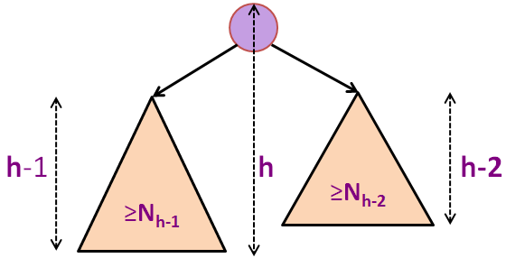
Pembuktiannya berdasarkan konsep dari Pohon AVL dengan ukuran-minimum dengan tinggi tertentu h.
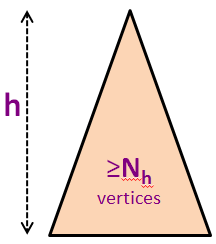
Biarlah Nh adalah jumlah minimum dari simpul-simpul dari sebuah Pohon AVL yang tinggi-seimbang dengan tinggi h.
Beberapa nilai-nilai pertama dari Nh adalah N0 = 1 (sebuah simpul akar tunggal), N1 = 2 (sebuah simpul akar dengan satu anak kiri atau satu anak kanan saja), N2 = 4, N3 = 7, N4 = 12, N5 = 20 (lihat gambar latar belakang), dan selanjutnya (lihat dua slide selanjutnya).
We know that for any AVL Tree of N vertices with height h (but not necessarily the minimum-size one), we have N ≥ Nh.
Example: In the background, we have N5 = 20 vertices but we know that we can squeeze 43 more vertices (up to N = 63) before we have a perfect binary tree of height h = 5.
Nh = 1 + Nh-1 + Nh-2 (formula untuk pohon AVL ukuran minimum dengan tinggi h)
Nh > 1 + 2*Nh-2 (karena Nh-1 > Nh-2)
Nh > 2*Nh-2 (tentu saja)
Nh > 4*Nh-4 (rekursif)
Nh > 8*Nh-6 (langkah rekursif lainnya)
... (kita cuma bisa melakukan ini h/2 kali, asumsi h awal adalah genap)
Nh > 2h/2*N0 (kita mencapai kasus dasar)
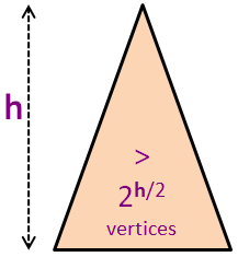
Nh > 2h/2 (karena N0 = 1)
N ≥ Nh > 2h/2 (menggabungkan dua slide sebelumnya)
N > 2h/2
log2(N) > log2(2h/2) (log2 di kedua sisi)
log2(N) > h/2 (penyederhanaan formula)
2 * log2(N) > h atau h < 2 * log2(N)
h = O(log(N)) (kesimpulan final)
Lihat BST contoh kembali. Lihatlah bahwa semua simpul-simpul adalah tinggi-seimbang, sebuah Pohon AVL.
Untuk dengan cepat mendeteksi apabila sebuah simpul v adalah tinggi seimbang atau tidak, kita memodifikasi invarian Pohon AVL (yang memiliki fungsi absolut didalamnya) menjadi: bf(v) = v.left.height - v.right.height.
Sekarang cobalah pada contoh Pohon AVL lagi. Beberapa simpul-simpul sepanjang jalur pemasukkan: {41,20,29,32} menambah tinggi mereka sebesar +1. Simpul-simpul {29,20} tidak akan lagi tinggi-seimbang setelah pemasukkan ini (dan akan dirotasi nantinya — akan dibahas di beberapa slide selanjutnya), yaitu bf(29) = -2 dan bf(20) = -2 juga. Kita perlu untuk mengembalikan keseimbangan.
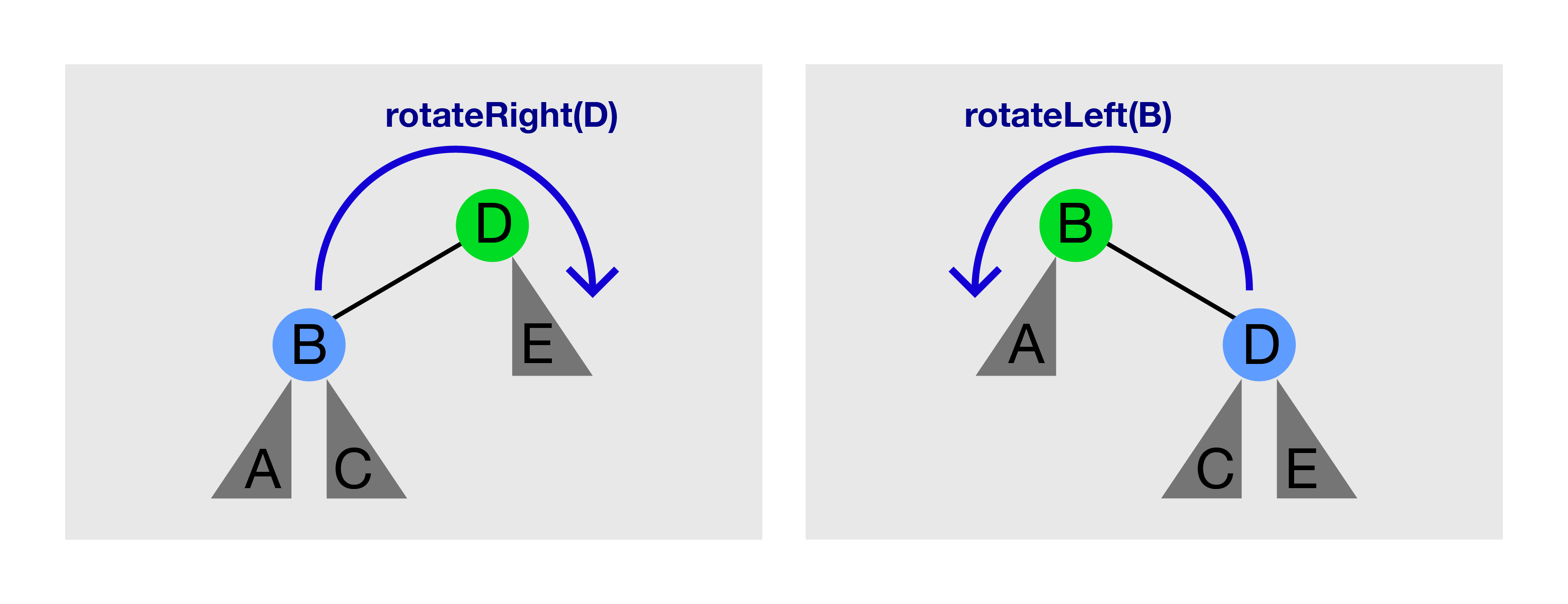
Lihatlah gambar diatas. Memanggil rotateRight(D) pada gambar di kiri akan menghasilkan gambar di kanan. Memanggil rotateLeft(B) pada gambar di kanan akan menghasilkan gambar di kiri lagi.
rotateRight(T)/rotateLeft(T) hanya bisa dipanggil jika T masing-masing memiliki anak kiri/kanan.
Rotasi Pohon menjaga properti BST. Sebelum rotasi, A < B < C < D < E. Setelah rotasi, lihatlah bahwa sub-pohon yang berakar pada C (jika ada) berpindah orangtua, tetapi A < B < C < D < E tidak berubah.
BSTVertex rotateLeft(BSTVertex T) // pra-syarat: T.right != null
  BSTVertex w = T.right // rotateRight adalah kopi terbalik dari ini
  w.parent = T.parent // metode ini susah bagi pemula
  T.parent = w
  T.right = w.left
  if (w.left != null) w.left.parent = T
  w.left = T
  // mutakhirkan tinggi dari T dan lalu w disini
  return w
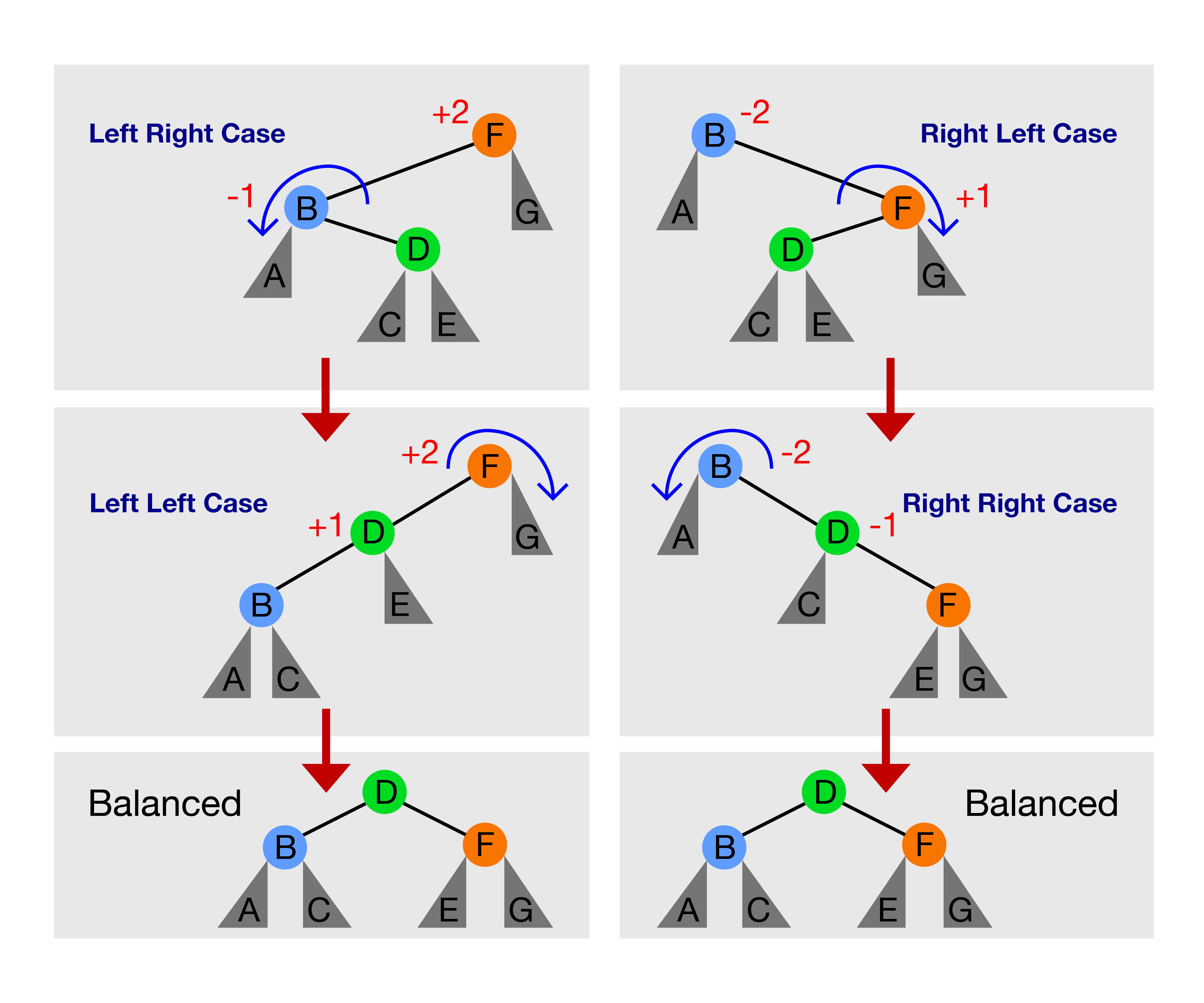
Hanya terdapat empat kasus berikut:
Diskusi: Apakah ada kasus-kasus rotasi pohon lainnya untuk operasi Masukkan(v) pada Pohon AVL?
Perbedaan utama dibandingkan dengan Masukkan(v) dalam pohon AVL adalah kita mungkin men-trigger satu dari empat kasus-kasus penyeimbangan yang mungkin beberapa kali, tetapi tidak lebih dari h = O(log N) kali :O, cobalah pada contoh diatas untuk melihat dua reaksi berantai rotateRight(6) dan lalu rotateRight(16)+rotateLeft(8).
We have now see how AVL Tree defines the height-balance invariant, maintain it for all vertices during Insert(v) and Remove(v) update operations, and a proof that AVL Tree has h < 2 * log N.
Therefore, all BST operations (both update and query operations except Inorder Traversal) that we have learned so far, if they have time complexity of O(h), they have time complexity of O(log N) if we use AVL Tree version of BST.
This marks the end of this e-Lecture, but please switch to 'Exploration Mode' and try making various calls to Insert(v) and Remove(v) in AVL Tree mode to strengthen your understanding of this data structure.
PS: If you want to study how these seemingly complex AVL Tree (rotation) operations are implemented in a real program, you can download this AVLDemo.cpp | java (must be used together with this BSTDemo.cpp | java).
Kami akan mengakhiri modul ini dengan beberapa hal-hal yang lebih menarik tentang BST dan BST yang seimbang (terutama Pohon AVL).
Untuk berbagai pertanyaan-pertanyaan lebih lanjut tentang struktur data ini, silahkan latihan pada modul latihan BST/AVL (tidak perlu login).
Tetapi, untuk pengguna-pengguna yang telah teregistrasi, anda sebaiknya login dan tekan ikon latihan dari halaman utama untuk secara ofisial menyelesaikan modul ini dan keberhasilan tersebut akan dicatat dalam akun pengguna anda.
Kami juga memiliki beberapa masalah-masalah pemrograman yang agak membutuhkan penggunaan struktur data BST yang seimbang ini (seperti Pohon AVL): Kattis - compoundwords dan Kattis - baconeggsandspam.
Cobalah mereka untuk mengkonsolidasikan dan mengembangkan pemahaman anda tentang struktur data ini. Anda diijinkan untuk menggunakan C++ STL map/set, Java TreeMap/TreeSet, atau OCaml Map/Set jika itu mempermudah implementasi anda (catat bahwa Python tidak mempunyai implementasi built-in dari BST seimbang).