Visualization of one of the simplest data structure in Computer Science: Array (and its sorted form) surprisingly has not been done in VisuAlgo since its inception 2011-January 2024...
Stay tuned while we improve this page and its features.
(Compact) Array is among the easiest and the most versatile data structure in Computer Science. Array is built-in almost all programming languages, e.g., C++, Python ('array' is called as 'list' in Python), Java, etc.
We can use (Compact) Array to implement List ADT.
We can use (Compact) Array to solve many classic problems. When not being used as a List ADT implementation (where positional order matters), it is often beneficial to first sort the elements first so that we can utilize faster algorithms.
Please see List ADT overview.
(Compact) Array is a good candidate for implementing the List ADT as it is a simple construct to handle a collection of items.
When we say compact array, we mean an array that has no gap, i.e., if there are N items in the array (that has size M, where M ≥ N), then only index [0..N-1] are occupied and other indices [N..M-1] should remain empty.
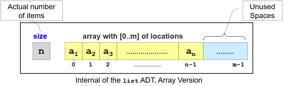
Let the compact array name be A with index [0..N-1] occupied with the items of the list.
get(i), just return A[i].
This simple operation will be unnecessarily complicated if the array is not compact.
search(v), we check each index i ∈ [0..N-1] one by one to see if A[i] == v.
This is because v (if it exists) can be anywhere in index [0..N-1].
Since this visualization only accept distinct items, v can only be found at most once.
In a general List ADT, we may want to have search(v) returns a list of indices.
insert(i, v), we shift items ∈ [i..N-1] to [i+1..N] (from backwards) and set A[i] = v.
This is so that v is inserted correctly at index i and maintain compactness.
remove(i), we shift items ∈ [i+1..N-1] to [i..N-2], overwriting the old A[i].
This is to maintain compactness.
get(i) is very fast: Just one access, O(1).
Another CS course: 'Computer Organisation' discusses the details on this O(1)
performance of this array indexing operation.
search(v)
In the best case, v is found at the first position, O(1).
In the worst case, v is not found in the list and we require O(N) scan to determine that.
insert(i, v)
In the best case, insert at i = N, there is no shifting of element, O(1).
In the worst case, insert at i = 0, we shift all N elements, O(N).
remove(i)
In the best case, remove at i = N-1, there is no shifting of element, O(1).
In the worst case, remove at i = 0, we shift all N elements, O(N).
The size of the compact array M is not infinite, but a finite number. This poses a problem as the maximum size may not be known in advance in many applications.
If M is too big, then the unused spaces are wasted.
If M is too small, then we will run out of space easily.
Solution: Make M a variable. So when the array is full, we create a larger array (usually two times larger) and move the elements from the old array to the new array. Thus, there is no more limits on size other than the (usually large) physical computer memory size.
C++ STL std::vector, Python list, Java Vector, or Java ArrayList all implement this variable-size array. Note that Python list and Java ArrayList are not Linked Lists, but are actually variable-size arrays. This array visualization implements this doubling-when-full strategy.
However, the classic array-based issues of space wastage and copying/shifting items overhead are still problematic.
There are various applications that can be done on a Compact (Integer) Array A:
See unsorted array and sorted array hints.
We will outline the possible actions that you can do in this page. For now, just try to guess based on the name of the function.
We will talk about the two modes: array (the content can be unsorted) versus sorted array (the content must always be sorted, without loss of generality: sorted in non-decreasing order).
There are already lots of (simple) applications that we can do with unsorted array.
There are better ways, especially if the array if sorted.
1There is a faster expected O(N) QuickSelect or O(N) worst-case linear time selection.
When the array is sorted, we open up a lot of possibilities.
There can be other ways.